Edge detection and processing using Canny edge detector and Hough transform

Why would you use traditional techniques in Computer Vision?

People often wonder whether there still is a need to study and use traditional Computer Vision (CV) techniques when Deep Learning (DL) seems to have superseded it. While DL has revolutionized CV and Artificial Intelligence (AI) in general, it certainly is not an all-around solution for every problem. While both approaches have their advantages and drawbacks, we will try to understand why using traditional techniques could still be beneficial.

The need for labelled datasets

For Neural Networks (NN) to learn and draw desirable insights, they usually need big amounts of data. Even for simpler problems, engineers need to go through the process of preparing and labeling the data. Typically, not only is it a complicated procedure, but also one that requires a lot of preprocessing, which frequently includes some traditional CV as well.

What's important to note is that even though NN can learn from smaller datasets, the accuracy of the model might be majorly affected. Thus, it is better to focus on traditional methods in some cases, especially when you have the necessary insight into the problem that you can transfer in a simple way into your algorithm.

The requirement of suficcient computational resources

Deep Learning models usually have millions of parameters inside, and every single one of them needs to be tuned during training. While it is generally seen as an advantage, allowing the model to understand very complex features of the image, this also means that the machine used for training has to be powerful enough to be trained in a practical time.

Whether we develop a solution in our workplace or for our own benefit, we have to consider that powerful computational resources not only bear a hefty price tag but also take their toll on the environment.

Deep Learning is sometimes just overkill

While the above arguments should be enough to consider traditional methods, it is worth noticing that NN models are sometimes just too much. Why bother with a process of preparing the data, acquiring and setting up the necessary computational resources, going through the process of adjusting the hyperparameters, if a problem looks relatively simple?

It is easy to get caught up in the hype of Deep Learning, but we must remember not to see Neural Networks as a golden hammer and every problem as a nail.

When all you have is a hammer, everything looks like a nail. – Abraham Maslow

Computer Vision techniques we will use

Before going through an example with code, it is important to understand the particular techniques used. We will use a Canny edge detector for detecting the edges in the image, Hough transform for finding straight lines, and dilation - one of the morphological operations - in between.

Morphological Operations

Morphological Operations are some of the most basic techniques in image processing, mainly used to process binary or grayscale images. When using a morphological operation, values of pixels in the output image are found by comparing the corresponding pixel in the input image with its neighbors. The size of the neighborhood is defined by a structuring element or kernel, but we will not go into much detail about it.

There are four primary morphological operations: Dilation, Erosion, Opening, and Closing, although we will only go through the two first, most basic ones.

Dilation

In dilation, the neighborhood patch aka kernel acts as a local maximum filter. This means that the value of the output pixel is equal to the maximum value of all pixels in the neighborhood of the input pixel. As a result, shapes present in the input image are being expanded on the output.

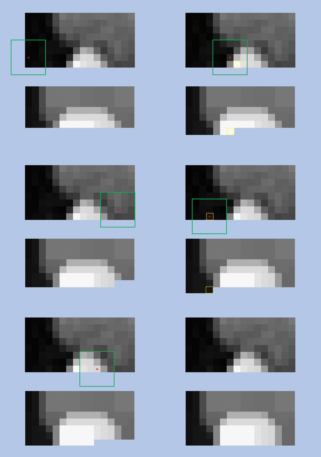
Erosion

It is an operation opposite to dilation - it reduces the shapes present in the input image instead. Its kernel acts as a local minimum filter - the value of the output pixel is equal to the minimum value of the input pixel neighborhood.

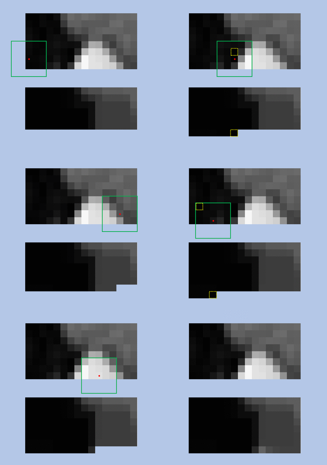
Sobel filter

Before we explain the Canny edge detection algorithm, it is helpful to understand how the Sobel filter works, as it is an algorithm that Canny heavily relies on.

Sobel filter is one of the most commonly used traditional algorithms for edge detection. It takes advantage of the fact that the edges are marked by large variations in pixel intensity.

Let's assume we have a 1D image. We can describe an edge as an observed change in intensity, as seen in the plot below:

What's more important for our technique is that the rise in intensity can be observed even more easily, once we plot the first derivative of the function mentioned above, since it represents the rate of change of one variable (in our case intensity) with respect to another variable (pixel location):

An important thing to note is that this works in both directions of the edge, as seen below:

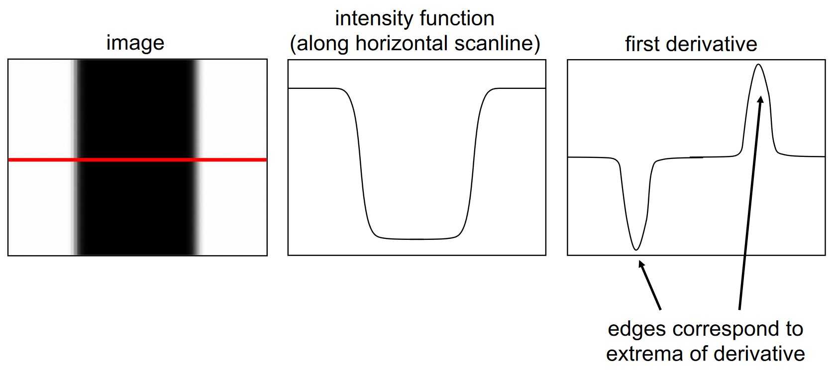
Now, what's remarkable about the Sobel filter, is that it takes advantage of this observation by detecting areas with high gradient! It detects these changes by approximating the derivative of the difference between each pixel and its surrounding pixels. Sounds familiar? It should! It is nothing else than a convolution with two particular kernels - one in the X direction and another in the Y direction:

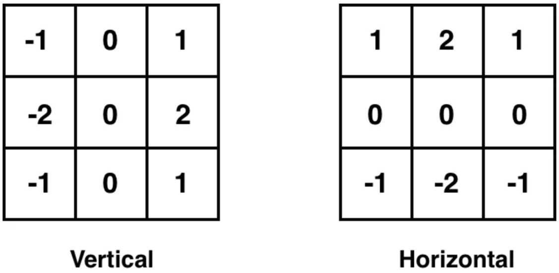
So essentially, with these kernels, we can calculate the value which tells us how "intense" the edge on a chosen pixel along the chosen axis is. The calculated values for each pixel using both vertical and horizontal kernels are summed to produce the final output image, containing information about the presence of edges in both directions, from the original image.

If you found yourself confused with how convolution works, I encourage you to take a look at Laura's post about Image recognition.

Canny edge detection

Canny edge detection is a multi-stage algorithm. It builds upon the Sobel filter idea with some additional stages, which we will now go over.

Noise reduction

Computer vision algorithms can be easily influenced by the noise present in raw image pixels, therefore usually it is recommended to reduce the noise beforehand. In Canny detector, we filter unnecessary noise with Gaussian blur. An example of Gaussian blur can be seen below:

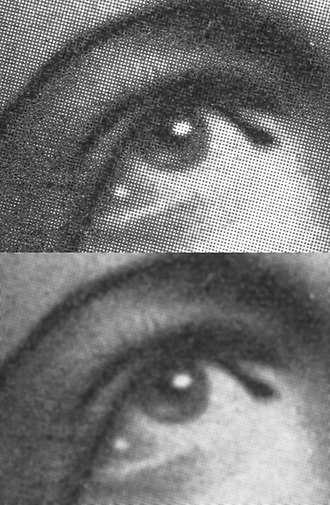
We will not go into much detail about Gaussian blur here, but it is important to note, that one has to tune noise filters. If we filter too much, we can loose important details - like our precious edges.

If you want to know more Gaussian filter, I recommend this well-written article.

Find intensity gradient of an image with Sobel filter

After we get rid of the noise, the image is then processed using a Sobel filter in both horizontal and vertical directions. Using these gradients, we can find the edge gradient value and its orientation for each pixel using the following equations:

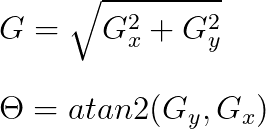
The gradient value is then rounded to the nearest 45-degree angle, representing vertical, horizontal, and two diagonal directions.

Non-maximum suppression

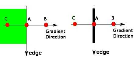
After finding the gradient values and directions, we want to eliminate any unwanted pixels (these which might not be part of the edge). We go through each pixel and compare it to its neighbors in the positive and negative directions. If the gradient value of the current pixel is greater than both neighbors, we leave it as a possible edge pixel. Otherwise, we set the value of the current pixel to zero. This is called non-maximum suppression.

Consider the example below. Point A is on the vertical edge, and points B and C are in gradient directions. If point A gradient magnitude is greater than both B and C (A forms a local maximum), it is considered an edge.

Hysteresis Thresholding

For the final stage, every pixel gradient magnitude is compared with two threshold values to decide if it is an edge pixel.

Let's call the threshold values minthresh and maxthresh, where minVal < maxVal. If an intensity gradient value is above maxVal, we consider it a strong edge, while values below minVal are excluded from the final result. For all the other pixels lying between these values, the decision is based on their association with strong edges (above maxVal). If they are connected to strong edge pixels, we accept them as part of the edge (they are called weak edges). Otherwise, we suppress them.

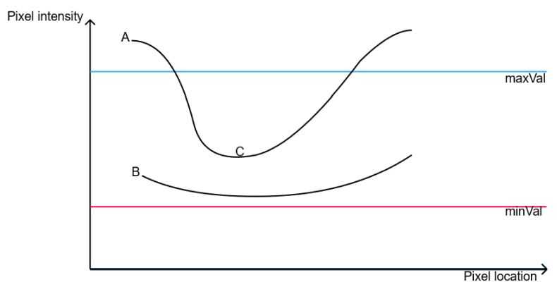
In the example above, A would be considered strong edge, B would be discarded and C would be considered weak edge based on it's connectivity to A.

Hough transform

Hough transform is an algorithm used to detect straight lines in images. It usually takes the output of an edge detection algorithm as an input (in our case, we use Canny for that).

To find lines in an image, the algorithm maps the edge points in an image onto the polar coordinate system. But what are polar coordinates?

Usually, we describe lines using the following formula: y = ax + b. However, in Hough transform algorithm, we may stumble upon a problem: when the line is vertical a = ∞ and our parameter space is unbounded. Therefore we describe each line using two parameters in the polar coordinate system: ρ and θ. ρ describes the shortest distance from the origin to the line, while θ is the angle between the x-axis and the perpendicular line representing ρ. In the polar system, for each point belonging to the line described using ρ and θ, the following equation is satisfied: ρ = x cos(θ) + y sin(θ)

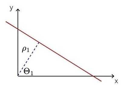
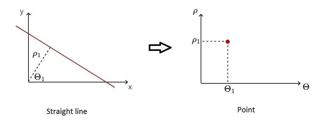
Therefore each straight line can be mapped as a point in the polar coordinate system, where the x-axis describes θ values and the y-axis represents ρ values.

Now, for every edge point, we can find multiple lines, each corresponding to one point in polar coordinates. What's really interesting about these points is that they form a sinusoid. It just comes from the fact that vector connecting the line with origin of the coordinate system must be perpendicular to the line (which length is ρ). Therefore when we change the angle, the p changes sinusoidally, because it revolves on a circle.

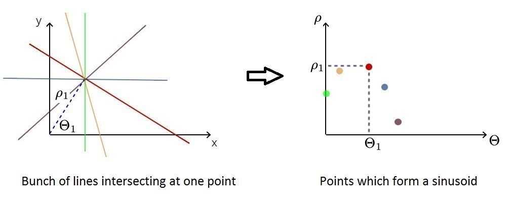
This allows us to represent each edge point (and lines intersecting in it) as a specific sinusoid in the polar system.

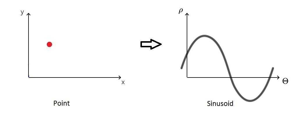
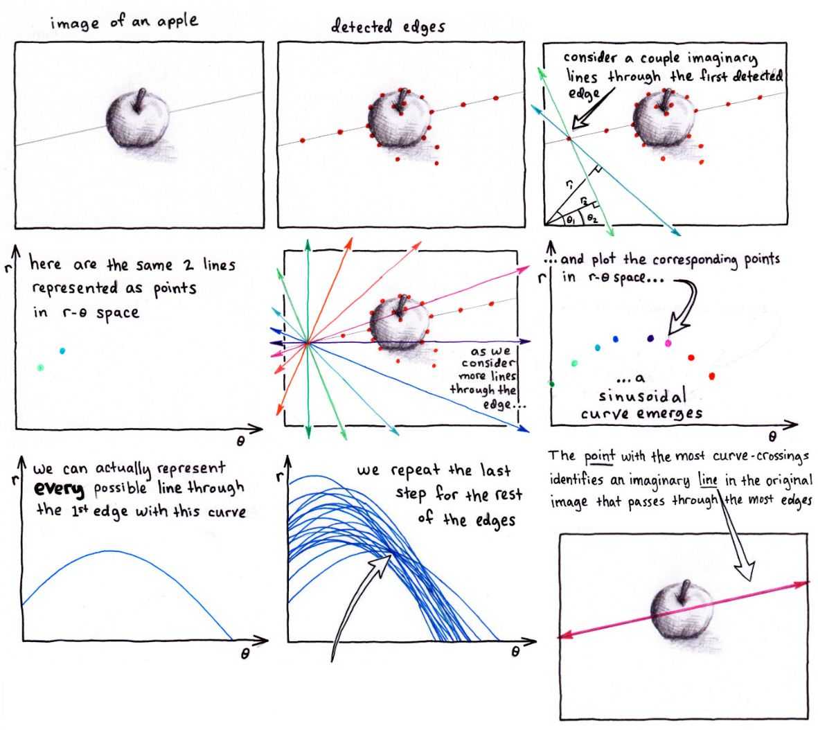
Now, how exactly can we begin to look for lines in the original edge image using this information? It turns out it's pretty straightforward - we have to seek for intersections between the sinusoids! So the algorithm will identify candidates for being a straight line and then accept only those with a number of intersections larger than a chosen threshold.

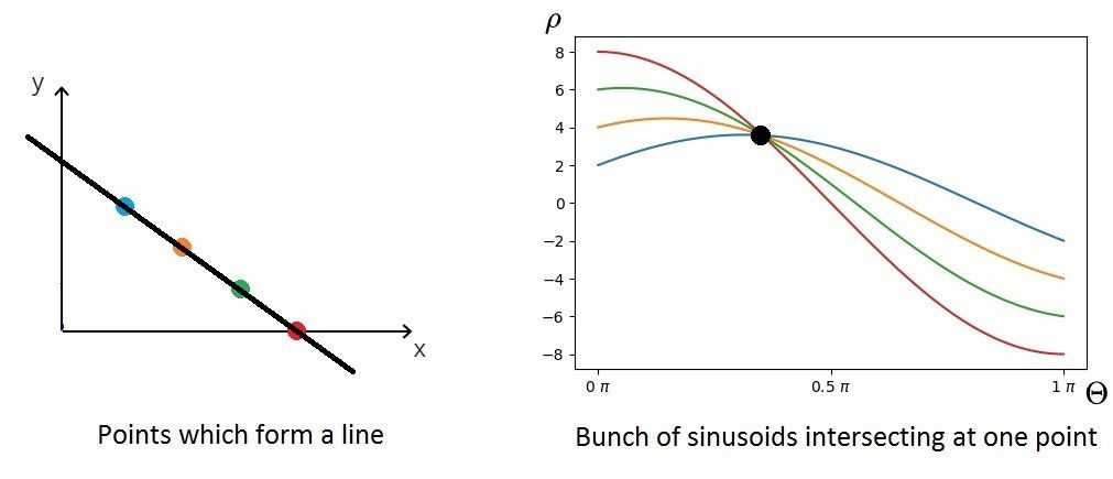
For a more detailed explanation I recommend reading the blog post by Tomasz Kacmajor, which is also the source of images used in an above explanation. I also highly recommend checking out the step-by-step visual explanation created by mlai on stack overflow:

Finding and filtering lines in a package template

Now that we have gone over the theory of techniques we will use, let's see how we can use them on an example problem we had at WTT.

Our input image was a package template, which will later be printed, cut out, and assembled. Our goal was to extract the main lines, which define the package outline and divide it into parts. We call those lines "dividers." We will work on an example seen below (left: input, right: output), where the "dividers" are shown in red:

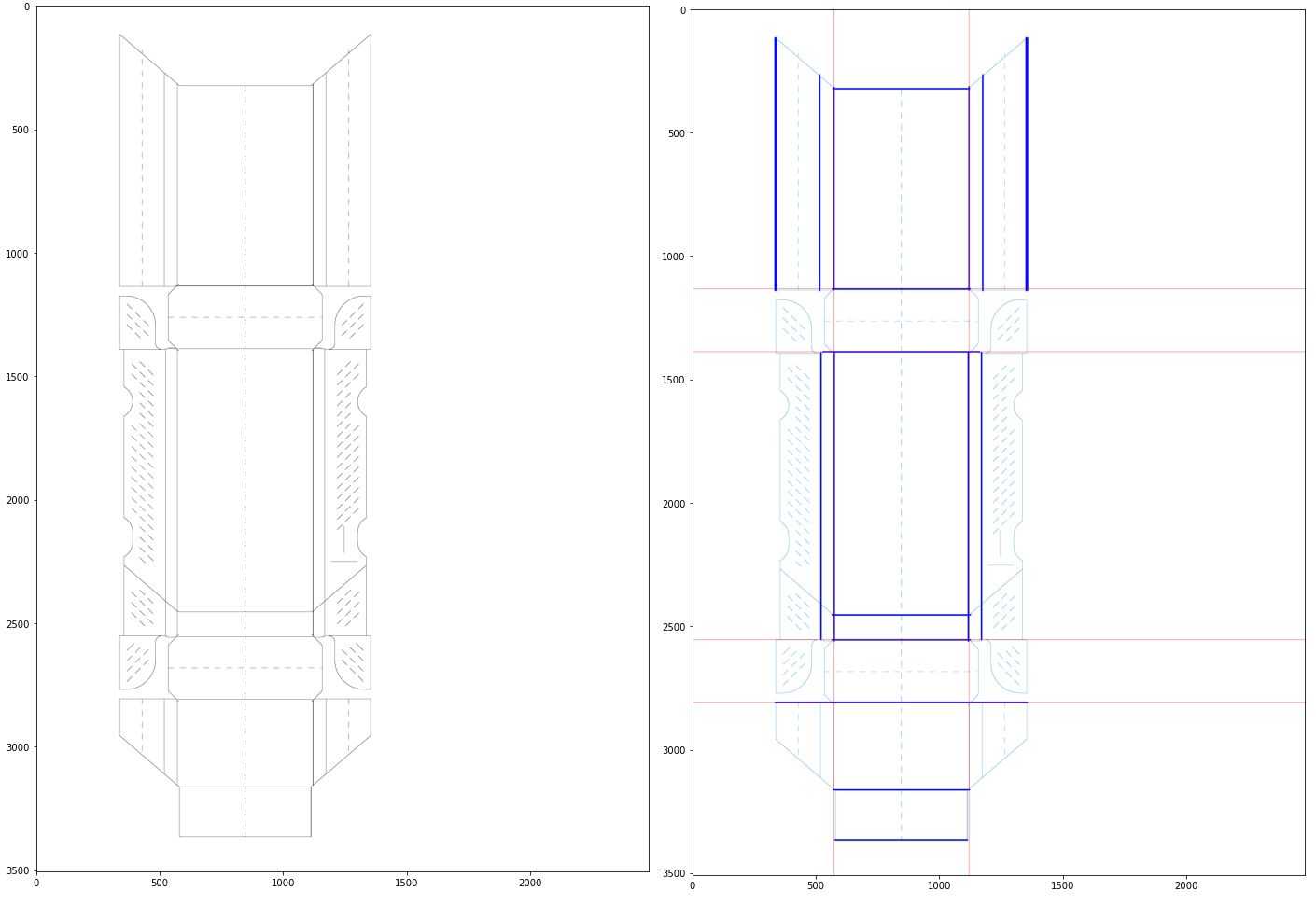
We will now go over the code step by step with visualizations in a following order:

1. The libraries used
2. Representing a line in Python
3. Detecting lines in our image
4. Filtering the detected lines
5. Finding the package divider lines

1. The libraries used

We mainly used NumPy for the mathematical operations and OpenCV for computer vision algorithms and image processing. We also used matplotlib for visualizing the images and found lines.

2. Representing a line in Python

Because in the major part of the code we will operate on lines, we created a helper class for easy access to:

• line beginning and end coordinates
• center of the line coordinates
• length of the line
• line angle relative to x axis

We also created the dist function which calculates euclidean distance between two lines centers.

We override the __hash__ function so we can create a set from a list of lines.

@dataclass
class Line:
    """
    Line object containing:
    - coordinates of its beginning and ending points,
    - coordinates of the center of the line
    - its length

    Functions:
    - angle - returns line orientation angle in radians
    - dist - euclidean distance between line centers
    """

    x1: int
    y1: int
    x2: int
    y2: int
    x_center: float = field(init=False)
    y_center: float = field(init=False)
    length: float = field(init=False)
    angle: float = field(init=False)

    def __post_init__(self):
        self.x_center = (self.x1 + self.x2) / 2
        self.y_center = (self.y1 + self.y2) / 2
        self.length = np.sqrt((self.x1 - self.x2) ** 2 + (self.y1 - self.y2) ** 2)
        self.angle = np.abs(np.arctan2(self.y2 - self.y1, self.x2 - self.x1))

    def dist(self, line: self) -> float:
        return np.sqrt(
            (
                (self.x_center - line.x_center) ** 2
                + (self.y_center - line.y_center) ** 2
            )
        )

    def __hash__(self):
        return hash(repr(self))

3. Detecting lines in our image

First we need to load our input image and convert it to grayscale. The reason behind it is that usually the separate R, G, B planes themselves do not contain any more distinct edge information than a single channel image, and this one is easier to operate on.

We also need to store the height and width of an image for later use.

gray = cv2.cvtColor(asset, cv2.COLOR_RGB2GRAY)
height, width = np.shape(gray)[:2]

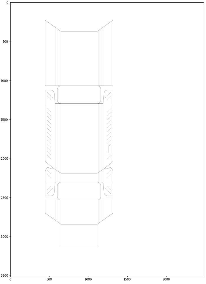
Next, we apply the Canny edge detector in just one line! The only parameters we need to pass are pixel values for the hysteresis thresholding procedure. In our case, the edge detector itself didn't do much since the image was already nicely prepared, but we always have to consider other possibilities where our image could not be that clean and well-prepared. For example, the package could be colored inside.

edges_canny = cv2.Canny(gray, threshold1=80, threshold2=120)

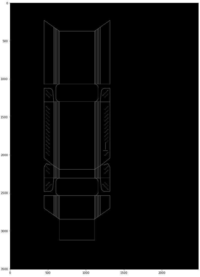
Now, we need to find vertical and horizontal lines in our image, but before we do that, we thought we should make the work a bit easier for Hough transform. We applied one of the morphological operators - dilation - to make the lines thicker, therefore, easier to find. This also prevents interpreting one line with minor distortion or a shift as two separate lines.

kernel = np.ones((5, 5), np.uint8)
edges_dilated = cv2.dilate(edges_canny, kernel)

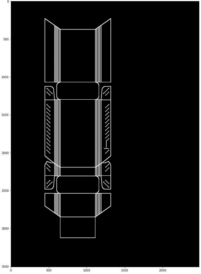
Now that we prepared our image, we can apply the Hough Lines algorithm with parameters tuned before-hand for our problem. Let's go over the parameters to see how to interpret them:

• rho - It defines the distance resolution of the accumulator in pixels. The lower the value, the bigger precision we get, which will ultimately give us more lines. We decided to set it to 1, which is pretty low, because we prefered to not miss any important line and just filter ones we don't need.
• theta - According to opencv documentation it is an "angle resolution of the accumulator in radians". In practice this means, that the larger theta we use, the less calculations of rho for each edge pixel are done. We use np.pi/2 since we only need two calculations: for vertical and horizontal lines.
• threshold - This is the parameter that defines how many intersections in the Hough space are enough to consider a line.
• minLineLength - Minimum line length.
• maxLineGap - Maximum allowed gap between points on the same line to link them.

lines = cv2.HoughLinesP(
    image=edges_dilated,
    rho=1,
    theta=np.pi / 2,
    threshold=100,
    minLineLength=450,
    maxLineGap=10,
)
lines = [Line(*line[0]) for line in lines]

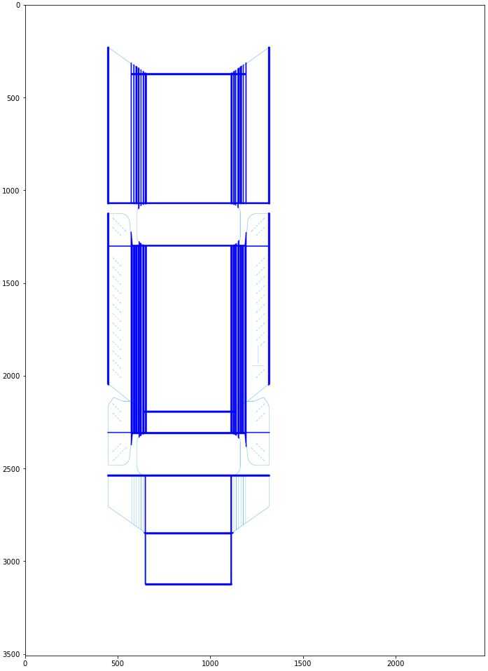
4. Filtering the detected lines

As we can see, after we detected all the horizontal and vertical lines that meet our requirements, there are still many unnecessary lines, and may prevent us from accurately recognizing the divider lines.

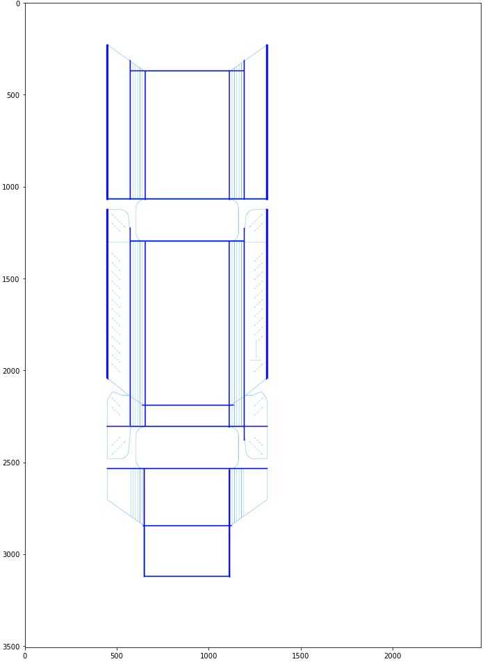
The most prominent problem is multiple vertical lines next to each other, but it is also important to notice that almost every line in this image is unusually thick. This happens because the lines in this image are several pixels wide and Hough transform actually detects them as multiple lines next to each other. Since we only need the most external lines, we decided it would be beneficial to filter the lines by the distance from one another.

First, we separate the vertical lines from horizontal ones using the angle property of the line:

def filter_and_group_lines_by_angle(lines: List[Line], margin: float=3*np.pi/180) -> Tuple[List[Line], List[Line]]:
    vertical = []
    horizontal = []
    for line in lines:
        if 0 - margin <= line.angle <= 0 + margin:
            horizontal.append(line)
        elif np.pi/2 - margin <= line.angle <= np.pi/2 + margin:
            vertical.append(line)
    return horizontal, vertical

horizontal_lines, vertical_lines = filter_and_group_lines_by_angle(lines)

Then we define a helper function to filter lines by distance. We go through a sorted list of lines one by one and append the current line to the filtered list only if the distance between the current line and all the other filtered lines is higher than the threshold.

def filter_lines_by_distance(sorted_lines: List[Line], min_distance: int):
    filtered = [sorted_lines[0]]
    for line in sorted_lines[1:]:
        if all([line.dist(line_) > min_distance for line_ in filtered]):
            filtered.append(line)
    return filtered

Finally, we filter the horizontal lines, with a previously hand-picked distance as a parameter:

horizontal_lines.sort(key=lambda line: line.y_center)
filtered_horizontal = filter_lines_by_distance(
    horizontal_lines, horizontal_max_dist=50
)

Since important horizontal lines are usually not that close to one another, we only need to use our function once, in the ascending y-value order. With vertical lines, have we considered only one direction, we would end up with these lines:

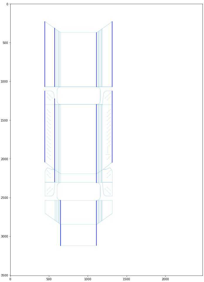
As we can see, in the case of the multiple vertical lines next to each other, only the leftmost ones remained, while we need to keep lines on both sides. Thus, we repeated the algorithm in both ascending and descending orders. Then, we merged the two lists of lines, using set mechanisms to prevent duplicates.

vertical_lines.sort(key=lambda line: line.x_center)
filtered_vertical_forward = filter_lines_by_distance(
    vertical_lines, vertical_max_dist=100
)
filtered_vertical_backward = filter_lines_by_distance(
    vertical_lines[::-1], vertical_max_dist=100
)
filtered_vertical = filtered_vertical_forward + list(
    set(filtered_vertical_backward) - set(filtered_vertical_forward)
)

As we can see, together with horizontal lines, the result is satisfactory:

5. Finding the package divider lines

The only thing left for us to do is to find the location of the "divider" lines based on the lines detected in the previous sections.

With horizontal lines, we have it easy. We have studied several assets with packages, and it turns out the number and order of the main horizontal lines is always the same. We can take advantage of this information by defining which indices of the sorted horizontal line list are we interested in. (negative indices are just counted from the end of a list)

horizontal_indices = [1, 2, -3, -4]

horiz_dividers = []
for idx in horizontal_indices:
    line = horizontal[idx]
    y = int(line.y_center)
    horiz_dividers.append(Line(0, y, width, y))

In case of vertical lines, considering different number and placement in various packages, we could not just define the chosen indices. In this case we decided to find the two vertical lines that are closest to the center in the upper 1/3 of the image.

# find center x of the package
vertical_top = [line for line in vertical if min(line.y1, line.y2) < height / 3]
vertical_top.sort(key=lambda line: line.x_center)
center_x = (vertical_top[0].x_center + vertical_top[-1].x_center) / 2

# find the index of the first line after the center
for i, line in enumerate(vertical_top):
    if line.x_center > center_x:
        idx = i
        break

# get the line before and after the vertical center
vert_dividers = []
for idx in [i - 1, i]:
    x = int(vertical_top[idx].x_center)
    vert_dividers.append(Line(x, 0, x, height))

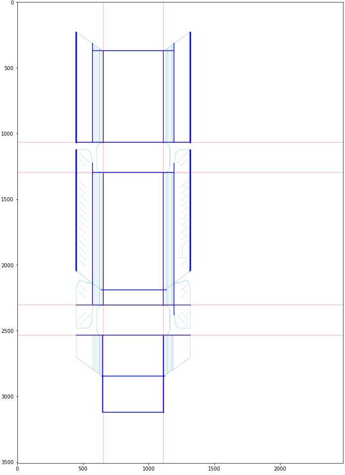
And there you have it! We found the coordinates of divider lines using only traditional computer vision methods. We can now easily locate specific parts of the package. It is worth mentioning that this whole process takes less than one second for an average asset!

Summary

People often forget that before the Deep Learning hype, there existed a lot of successful and very capable traditional computer vision techniques. In this post, we've presented and explained only a few of those: Sobel filter, Canny edge detection, Hough transform, and Morphological operations. We proved that these and other techniques can be used with success in some problems without the need to use AI and Neural Networks. We also presented a real-life example with code and results.