Optimize anything with hyperopt

In maths, computer science, and related fields, an optimization problem is a very broad term encompassing any problem where the aim is to find the best solution among all possible ones. Such a definition also entails a need for a common criterion that is used to judge each proposed solution, so that it's possible to choose the best one. In practice, there might be multiple such solutions, with equal values of the performance metric.

We can distinguish local optimization, where the solution found is the best one only for a subset of all possibilities, and global optimization, where the goal is to find the optimal solution for the whole search space. In this post, we'll strive for global optimization, which is significantly harder than finding local optimums. Depending on the nature of the problem, we can further divide optimization into continuous optimization and discrete optimization.

Continuous optimization

In continuous optimization, we search for a value of a continuous function as our solution. Training neural networks fall into this category. We use a continuous loss function to evaluate a solution that can be represented as a continuous vector of the network's weights. Due to this, it's possible to make arbitrarily small changes to the current solution, getting closer and closer to the optimum. The changes are dictated by the gradient of the loss function, so it's also essential for the function to be continuous and differentiable. For instance, in the problem of classification, the metric we usually care most about is accuracy, but it can't be used as a loss function since it's not differentiable. To circumvent this issue, we resort to a surrogate function in the form of logistic loss.

Discrete optimization

Discrete optimization is a different beast. In this scenario, the solution we are looking for is not continuous and can be, for example, an integer, a graph, a selection of set elements, and more. What's characteristic in such problems is that the possible solutions form a countable set. It doesn't necessarily mean that there's a finite number of them, rather, that they can be "enumerated" (for details, refer to the definition of countable infinity). In discrete optimization, a loss (or objective) function is still used to score solutions, but as the solutions are not continuous, they are not updated based on the objective function gradients. This allows for the usage of a wider spectrum of different metrics.

In this post, we'll focus on discrete optimization. Due to the fact that it doesn't require the solution to be continuous, it can be adopted to lots of diverse problems that wouldn't suit continuous optimization. A surprisingly high number of problems we encounter in our daily lives could be stated as a discrete optimization problem. For example, selecting the order of daily tasks, the kind of bread to buy, a route to work - each of these could be formulated as a discrete optimization problem. Each time you face a problem of selecting one of a few options - you are performing a discrete optimization. This also applies to typical engineering work - which algorithm to use, what parameters to chose, how many CPU cores you will need, the number of retries after an unsuccessful operation, and more.

Usually, the choice we make is based on our past experience, knowledge of others, established practices, or simply gut feeling. Such heuristics work fine in most cases. Their unquestionable advantage is the fact that they minimise the decision time. Often we wouldn't want to spend countless hours testing various solutions just to gain a minor improvement of the quality we care about. However, what if we could defer this decision process to an automated tool, which could test various scenarios for us, and ideally, do it in a smart fashion, testing the most promising solutions based on the past results? This is where libraries such as hyperopt come into play.

Methods

There are multiple methods to solve discrete optimization problems. The simplest one being simply testing each feasible solution and picking the best one according to the defined criterion. Such an approach guarantees arriving at the optimum, but it is practical only for small search spaces. The number of possible solutions is often overwhelmingly high, making it impossible to check all of them in a reasonable time.

The second easiest option would be to perform a grid search. In this version, we check only a subspace of solutions. This method is quite versatile since we can control the number of checked solutions. The greater the number, the greater the chances of arriving at an optimal or near-optimal one. In the case of the grid search, the solutions are checked in a grid-like fashion, where they are evenly spaced. For example, if the optimized parameter is a single number, we could for instance check the solutions in a sequence like 0, 5, 10, 15.... A similar technique, called simply a random search, doesn't have this property. The solutions are drawn from a random distribution, and an example sequence could look like 31, 2, 13, -1....

There are multiple other options for solving discrete optimization problems. If a problem can be divided into sub-problems for which optimal solutions can be found, dynamic programming approaches can be used. If, when traversing some solution we can determine that it can't be better than a solution we've already checked, backtracking can be implemented.

There is also quite a diverse set of possible heuristic methods to choose from, some of which are inspired by mechanisms observed in nature. This category includes techniques like hill climbing, genetic programming, ant colony optimization, or simulated annealing. Unlike random algorithms, these methods try to utilize smart tricks together with the information of a solution structure and its quality to check the most promising solutions, instead of doing it blindly.

Hyperopt

According to the docs, "hyperopt is a Python library for serial and parallel optimization over awkward search spaces, which may include real-valued, discrete, and conditional dimensions". This short description neatly sums up the library's powerful capabilities. It can, based on a user-defined loss function and a search space, perform optimization of complex functions. It supports a wide range of parameter types - they can be continuous or discrete, strictly conditional or combinatorial. This versatility makes hyperopt a versatile tool suited for usage in lots of different contexts.

Hyperopt supports two ways of traversing the solutions space in search of the optimal solution - grid search or Tree of Parzen Estimators (TPE). You can read up on them in Algorithms for Hyper-Parameter Optimization. In a nutshell, the tree-based method tries to pick the most promising solutions for tests, potentially arriving at the optimum quicker than the random search. However, it is more susceptible to falling into local optima. It's probably best to experiment with all three methods or pick one based on your problem characteristics.

Another interesting aspect of the tool is the fact that it exists in four versions:

• hyperopt - the general one
• hyperopt-nnet - for optimizing neural nets hyperparams
• hyperopt-convnet - for optimizing convolutional neural nets hyperparams
• hyperopt-sklearn - for use with scikit-learn estimators

If you want to get all the details, refer to the official documentation of the tool.

Experiments

Having familiarized ourselves with the basic theory, we can now proceed to make use of hyperopt in real-world problems. The sections below present two use cases of the library - the first one being a very concise model and hyperparameters selection for scikit-learn, and the second one a search for optimal preprocessing for optical character recognition (OCR). You can find all the code used in the following snippets in this GitHub repository.

Hyperparameters optimization in machine learning

Let's begin with a simple usage with scikit-learn. We'll use a sample dataset and let hyperopt choose the optimal estimator and its parameters to arrive at the best solution. The dataset loaded is the Iris plants dataset, which represents a simple classification problem. The code below downloads the dataset, splits it into train and validation subsets, and then, with neither a model type nor hyperparameters specified manually, trains an effective estimator. At the very end, the final accuracy on the validation set is calculated, and the details of the best model found are presented.

from hpsklearn import HyperoptEstimator
from hyperopt import tpe
from sklearn.datasets import load_iris
from sklearn.model_selection import train_test_split

# Loading the data:
X, y = load_iris(return_X_y=True)
X_train, X_test, y_train, y_test = train_test_split(
    X, y, test_size=0.2, random_state=123
)

# Defining and training the estimator:
estim = HyperoptEstimator(algo=tpe.suggest, max_evals=100, trial_timeout=60)
estim.fit(X_train, y_train)

# Final accuracy and details of the best model:
score = estim.score(X_test, y_test)
print(f"Accuracy of the best model: {score}")

model = estim.best_model()
print(f"Details of the best model:\n{model}")

Output:

>>> 100%|██████████| 100/100 [00:01<00:00,  1.93s/trial, best loss: 0.04166666666666663]
>>> Accuracy of the best model: 0.9666666666666667
>>> {'learner': ExtraTreesClassifier(criterion='entropy', max_features=0.05226290949574741,
     n_estimators=46, n_jobs=1, random_state=3, verbose=False), 'preprocs': (Normalizer(),), 'ex_preprocs': ()}

We can see that the accuracy is pretty satisfactory (more than 96% with 4 classes), although the problem at hand is relatively simple. An interesting point to note is the fact that the library specified preprocessing steps (under preprocs key) along with the model type and its parameters (specified by learner). Thus, it handles all the stages of a typical ML training pipeline and can be said to be an automated machine learning (AutoML) solution. To see an alternative implementation of AutoML in the H2O library, check out Painless machine learning with AutoML.

Preprocessing optimization for OCR

The experiment above serves as the simplest example for hyperopt-sklearn. It has proved that it's possible to train an effective model by delegating all the hard work to a TPE-based hyperopt estimator. This use case, while fancy, is somewhat limited. I stated above that discrete optimization problems can be found everywhere. Let's try optimizing something less obvious - preprocessing steps for OCR.

Dataset

Let's say I want to create a mobile app that would snap a picture of an inspiring excerpt from a book and translate it into a text form so it can be used as an Instagram caption. Some example pictures may look like this:

OCR engine

To convert images into text, we'll use Tesseract OCR - an open-source OCR engine. It can be used in Python with pytesseract. Let's see the results of OCR for the two images above:

import cv2
import pytesseract

for img_path in ['1.jpg', '2,jpg']:
  img = cv2.imread(img_path)
  print(pytesseract.image_to_string(img, config="--psm 6"))

Output:

>>> Iam like a fish
    in love with a bird
    wishing I could fly
>>> this nice lifestyle that I have? What are all the Pixar shai
    to think? I talked to people I respected. I finally called Be
    about eight one Saturday morning—too early. I gave him | v

We can see that the first image was read almost perfectly, the only mistake being a lack of space between "I" and "am". The situation is much worse for the second excerpt. The text on the right-hand side of the image was read incorrectly or not seen at all. This can probably by explained by a low contrast in this area of the picture. This is a disappointing result, but, fortunately, not all hope is lost. In the official documentation of Tesseract, there's a document titled Improving the quality of the output listing some tricks and tips on how to make images easier to read by the OCR engine. The hints include preprocessing steps like rescaling, binarisation, denoising, and more.

There's a snag, however. Most, if not all, of the preprocessing steps listed in the document are parametric. How are we to know what parameters to use to get optimal results? Some of the methods, like fastNlMeansDenoising() used to remove noise from the image, have some recommended values as defaults. They might serve as good starting points, but it's not unreasonable to think that they could be fine-tuned to receive superior results. This is an excellent opportunity to let hyperopt pick the parameters for us!

Objective function

To start the optimization process, we need an objective function used to gauge the OCR performance. Put simply, we want to compare the text read by OCR with the expected text, provided by us. A reasonable metric for our needs would be the Levenshtein distance (also known as the edit distance), which is the minimum number of single-character edits required to make two strings equal. The distance between "horse" and "house" is 1, while the distance between "java" and "python" is 6. The way the Levenshtein distance is implemented is interesting on its own and is a neat example of dynamic programming, but, to keep things simple, we'll make use of an existing library called python-Levenshtein. You can find its GitHub repository here. All method definitions can be found in the documentation. The edit distance is available under distance(string1, string2) function. We could use it, but it's probably better to use ratio(string1, string2) because it returns a normalized similarity between the two strings (the value is between 0 and 1), thus the result is easier to interpret. Let's test it:

from Levenshtein import distance, ratio

print(f"Distance between horse and house is {distance('horse','house')}")
print(f"Distance between java and python is {distance('java','python')}")

print(f"Similarity between horse and house is {ratio('horse','house')}")
print(f"Similarity between java and python is {ratio('java','python')}")

Output:

>>> Distance between horse and house is 1
>>> Distance between java and python is 6

>>> Similarity between horse and house is 0.8
>>> Similarity between java and python is 0.0

The similarity metric makes it clear that "java" has nothing to do with "python", while "horse" is somewhat similar to "house". Nice.

Preprocessing

Now, with some sample images and texts, we can start optimizing! We want hyperopt to go over a lot of potential preprocessing scenarios and fish out the best one for us. A very interesting aspect of using hyperopt is that it's not limited to searching over a range of numerical values. The search space passed to hyperopt has a graph structure, meaning that you can define conditional parameters. This is great for our use case. Let's say, based on the Tesseract docs, that we want to consider the following preprocessing operations:

• scaling
• binarization
• denoising
• erosion
• dilation

However, it might turn out that the optimal preprocessing includes only a subset of these operations. For instance, maybe eroding the image is not beneficial at all and we should skip it. Furthermore, some operations make sense only if some other ones were performed. Both erosion and dilation can be applied to a binarized image only, so they shouldn't be considered if no binarization was executed.

Implementation-wise, we'll use the following functions available in OpenCV:

• resize() for scaling
• adaptiveThreshold() for binarization
• fastNlMeansDenoising() for denoising
• erode() for erosion
• dilate() for dilation

Hyperopt search space

The preprocessing methods mentioned above accept some integer parameters that we will pick with hyperopt. Let's define the search space for our problem:

search_space = {
    "resize": hprange("resize", 50, 200), (1)
    "binarize": hp.choice( (2)
        "binarize",
        [
            (
                True, (3)
                (
                    hp.choice(
                        "binarize_algorithm",
                        [cv2.ADAPTIVE_THRESH_GAUSSIAN_C, cv2.ADAPTIVE_THRESH_MEAN_C],
                    ),
                    hprange("binarize_blocksize", 13, 29, 2),
                    hprange("binarize_c", 7, 15),
                ),
                {
                    "dilate": hp.choice( (4)
                        "dilate", [(True, hprange("dilate_kernel", 1, 4, 2)), (False,)]
                    ),
                    "erode": hp.choice( (5)
                        "erode", [(True, hprange("erode_kernel", 1, 4, 2)), (False,)]
                    ),
                },
            ),
            (False,), (6)
        ],
    ),
    "denoise": hp.choice( (7)
        "denoise",
        [
            (
                True, (8)
                (
                    hprange("denoise_h", 1, 10, 2),
                    hprange("denoise_windowsize", 13, 27, 2),
                    hprange("denoise_blocksize", 5, 15, 2),
                ),
            ),
            (False,), (9)
        ],
    ),
}

The code above uses methods like hp.choice() and hp.randint() (inside hprange()) to specify the options and ranges for different parameters. You can see the exact definitions of all possible parameter expression functions in the documentation. The helper method hprange() is meant to be a wrapper for hp.randint() and work similarily to native range() function in Python. It's defined in the following way:

def hprange(name, start, stop, step=1):
    interval = stop - start
    stop = math.ceil(interval / step)
    return start + hp.randint(name, stop) * step

With hprange() it's possible to specify the range of a parameter, together with a step between consecutive values. This is especially handy for parameters accepting only odd or even values - in this case, it's enough to specify step=2 when calling the method.

Let's go back to the search space definition.

The code looks a bit contrived, but, in reality, it's rather simple. The complexity stems from conditional branches in the search space. An alternative would be to specify all parameters in a flat way, and simply ignore them in the objective function if they are not used. This, however, is suboptimal as can be read in the documentation:

Whenever it makes sense to do so, you should encode parameters as conditional ones this way, rather than simply ignoring parameters in the objective function. If you expose the fact that 'c1' sometimes has no effect on the objective function (because it has no effect on the argument to the objective function) then search can be more efficient about credit assignment.

With search space defined, we can use hyperopt.pyll.stochastic.sample() to sample from it. Let's check some random paramaters combinations:

for _ in range(5):
    print(hyperopt.pyll.stochastic.sample(search_space))

Output:

>>> {'binarize': (False,), 'denoise': (True, (1, 13, 13)), 'resize': 99}
>>> {'binarize': (False,), 'denoise': (True, (1, 23, 7)), 'resize': 175}
>>> {'binarize': (True, (0, 27, 14), {'dilate': (False,), 'erode': (False,)}), 'denoise': (False,), 'resize': 151}
>>> {'binarize': (False,), 'denoise': (True, (5, 21, 5)), 'resize': 106}
>>> {'binarize': (True, (1, 23, 9), {'dilate': (True, 1), 'erode': (False,)}), 'denoise': (True, (7, 15, 11)), 'resize': 97}

Looks good. We can see that we received somewhat random combinations of preprocessing steps. These will produce distinct images, leading to different OCR results

Hyperopt objective function

With the search space defined, we can create fully parametric versions of the preprocessing methods:

import cv2
import numpy as np


def resize(img, params):
    height = params["resize"]
    return cv2.resize(img, (int(img.shape[1] * height / img.shape[0]), height))


def binarize(img, params):
    if params["binarize"][0]: (1)
        args = params["binarize"][1] (2)
        img = cv2.adaptiveThreshold(
            img, 255, args[0], cv2.THRESH_BINARY, args[1], args[2] (3)
        )
    return img


def denoise(img, params):
    if params["denoise"][0]:
        args = params["denoise"][1]
        img = cv2.fastNlMeansDenoising(
            img,
            None,
            h=float(args[0]),
            templateWindowSize=args[1],
            searchWindowSize=args[2],
        )
    return img


def erode_and_dilate(img, params):
    if params["binarize"][0]:
        args = params["binarize"][-1]
        if args["erode"][0]:
            kernel_size = args["erode"][1]
            kernel = np.ones((kernel_size, kernel_size), np.uint8)
            img = cv2.erode(img, kernel)
        if args["dilate"][0]:
            kernel_size = args["dilate"][1]
            kernel = np.ones((kernel_size, kernel_size), np.uint8)
            img = cv2.dilate(img, kernel)
    return img

We pass a dictionary params to each function. The function should be aware of how to extract its specific parametrization and perform actions based on it. As an example, consider binarize():

Other methods work in much the same fashion. Combining them all in a single preprocessing pipeline results in the following code:

import cv2
import pytesseract
from preprocessing import binarize, denoise, erode_and_dilate, resize

def _ocr(img_path, params):
    # Reading the image + converting to grayscale:
    img = cv2.imread(img_path)
    img = cv2.cvtColor(img, cv2.COLOR_BGR2GRAY)

    # Parametrized transformations:
    img = resize(img, params)
    img = binarize(img, params)
    img = denoise(img, params)
    img = erode_and_dilate(img, params)

    # OCR:
    text = pytesseract.image_to_string(img, config="--psm 6").strip()
    return text, img

The final step is creating the objective function:

import re
from Levenshtein import ratio
from plotting import display_ocr_result

def dissimilarity(img_path, text_path, params, display=False):
    ocr_text, preprocessed_img = _ocr(img_path, params)
    with open(text_path) as file:
        expected_text = re.sub("\s+", " ", file.read().strip())
    similarity = ratio(re.sub("\s+", " ", ocr_text), expected_text)
    if display:
        display_ocr_result(ocr_text, preprocessed_img, similarity)
    return 1 - similarity

This function reads the image from img_path and the expected text from a text file under text_path. It also accepts a dictionary of params that is later passed to the OCR method. The final similarity is calculated with ratio() and turned into dissimilarity defined as 1- similarity. We do this since hyperopt tries to minimize loss/objective functions, so we have to invert the logic (the lower the value, the better).

We can check the effects of different parameters on a single image with:

for _ in range(2):
    params = hyperopt.pyll.stochastic.sample(search_space)
    print(params)
    dissimilarity('data/images/8.jpg', 'data/texts/8.txt', params, display=True)

Outputs:

>>> {'binarize': (False,), 'denoise': (False,), 'resize': 127}

>>> {'binarize': (True, (0, 19, 13), {'dilate': (False,), 'erode': (True, 3)}), 'denoise': (False,), 'resize': 100}

The results are interesting. As can be seen, the second example was read by Tesseract with a much higher accuracy. In the first example, the only operation applied was resizing. In the latter image, binarization and erosion was additionally performed, which proved beneficial for this partuclar image. Is it possible that the results might be even better?

Final optimization

We now have all the pieces to perform the optimization. However, to make the results most robust, we would like to perform the analysis on more than one or two images. Due to this, we define a cumulative_dissimilarity() method, which sums up the OCR losses for all images under a given directory. In this particular case, I prepared eight images, which can be seen here.

from glob import glob
from pathlib import Path
from hyperopt import STATUS_OK

def cumulative_dissimilarity(params, directory="data", display=False):
    total_loss = 0
    images_dir = Path(directory) / "images"
    texts_dir = Path(directory) / "texts"
    for image in glob(str(images_dir / "*.jpg")):
        text = texts_dir / (Path(image).stem + ".txt")
        total_loss += dissimilarity(image, text, params, display=display)

    return {"loss": total_loss, "status": STATUS_OK, "params": params}

This is the method that will be directly passed to hyperopt. Note that we return a dictionary structure, where under "loss" we pass the final value of the objective function. Under "params", we store the parameters so it's possible later to look at the history of evaluated parameters.

Let's proceed to the optimization:

from hyperopt import Trials, fmin, hp, space_eval, tpe

trials = Trials()
best = fmin(
    cumulative_dissimilarity,
    search_space,
    algo=tpe.suggest,
    max_evals=4000,
    trials=trials,
)

We pass the cumulative_dissimilarity method, together with the previously defined search_space. The adaptive TPE algorithm is used to choose consecutive parameters. The limit of solutions checked is set to 4000 - this number should be a reasonable trade-off between the processing time and the accuracy of the final result. Finally, we use trials to store the history of evaluation.

The output of the code above is the following:

>>> 100%|██████████| 4000/4000 [3:03:59<00:00,  2.76s/trial, best loss: 0.2637919640168027]

As can be seen, it took 3 hours to test 4 thousand samples, and the lowest loss achieved is around 0.26. The history of tested parameters and their corresponding losses is saved under trials variable. Let's plot the losses over time with a simple utility function:

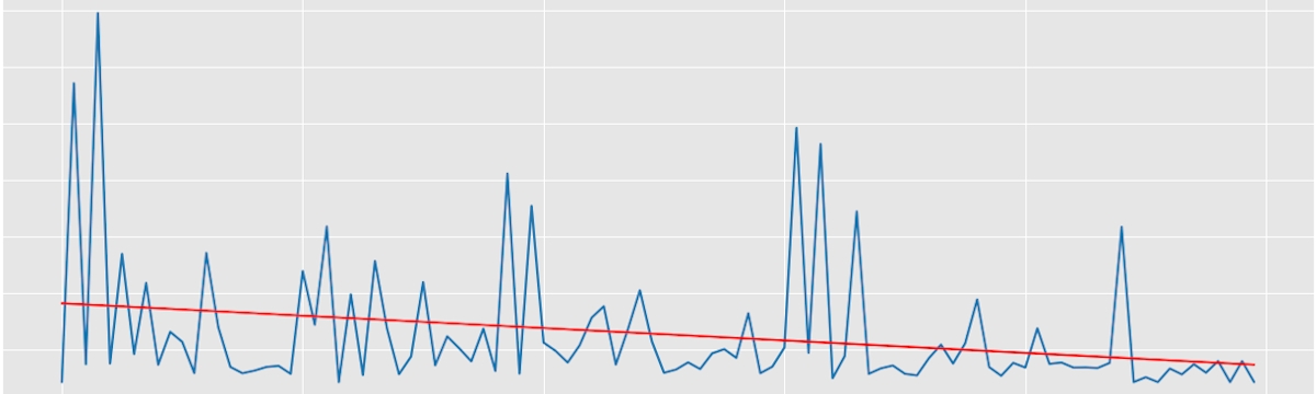
plot_losses_history(trials.results, (0.25, 1.5))

As can be seen, the loss history is pretty noisy. Due to this, a linear regression line fitted to the losses is added to the plot in red colour. The regression line is decreasing, signifying that the trend was for the loss to get lower over time. This is a characteristic of the algorithm we've used - Tree of Parzen Estimators. Was the optimization random, we would expect a straight, horizontal line.

Let's see what the best parameters are with space_eval():

params = space_eval(search_space, best)
print(params)

Output:

>>> {'binarize': (True, (0, 27, 8), {'dilate': (True, 1), 'erode': (False,)}), 'denoise': (False,), 'resize': 181}

We can see that out of five preprocessing methods, three were used: binarization, dilation, and resizing. The exact parameters used are displayed as well.

Let's check the results of such preprocessing on some images. You can check the results for all eight images in this noteboook.

We can see that the results are not ideal, but they still look pretty satisfactory. The first image was read perfectly, while the remaining three contain some minor errors. This is, however, the best result (when it comes to the average error) that the method was able to find. And the best thing is, the optimization process took place automatically, taking the effort of tuning the parameters off our shoulders.

Summary

Finding optimal solutions for hard problems often seems like an insurmountable challenge. In this post, we've shown that with a well-defined search space and an objective function, it is possible to defer to automatic solutions like hyperopt. The versatility of the tool makes it an apt choice for tuning parameters, choosing the optimal algorithm, finding the best permutations, and much more. The effort exerted when formulating the problem and possible solutions is bound to pay off in both the quality of the final solution and the time it takes to arrive at it.