Have you ever wondered if deep learning is for you? You feel that you don't know math enough to understand what it is about or thought you need a supercomputer to train neural networks? Well, it's not entirely true. Some time ago, I took part in the Fast.AI online course that teaches deep learning in a way that differs from most of the online courses available. Instead of deep diving into math theory, it starts from the top, from building end to end application and explaining each concept one by one. In this article, I will follow the same path, and I will show you what it is by building an end-to-end application of the image classifier and explaining the most essential concepts. You will find that understanding of these concepts does not necessarily require a PhD in math as they are pretty simple, and most of the time, they just sound scary.
What is Deep learning ?
Deep learning is part of a broader family of machine learning methods. According to Wikipedia:
Machine learning (ML) is the study of computer algorithms that improve automatically through experience. It is seen as a part of artificial intelligence.
To better understand what it means, let's take a step back and think about how a typical computer program works.
In a typical program, we have:
- Inputs, e.g. numbers, text, images
- The program that is receiving inputs and executes a codified algorithm for our task. And this is something we have to figure out by ourselves. We need to code here how to treat input data to produce our desired outputs.
- Finally, we have an output of the program.
If you are a programmer, you already know all of that. You do it almost every day in your projects. But usually, the stuff you're implementing is a relatively easy task. But what if you have a complex task that it is nearly impossible to find out the algorithm to code. What if you wanted to have a program that plays checkers game, recognizes objects in input images or translates the language of the given text. It is challenging to figure out such an algorithm and even impossible in some cases. But there is a way to accomplish that task, and the idea is, in fact, quite old.
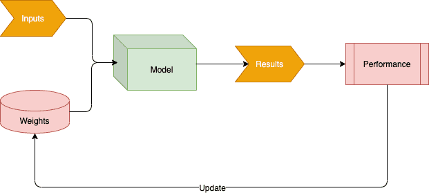
In the 1960s, the researcher Arthur Samuel showed a different way of solving complex tasks. He also created a program to play checkers that beat the state champion that time. His idea can be depicted below.
- Together with the inputs, which could be images, text files or positions of pieces in a checker game, we have weights that feed the model (program)
- The results of our program could be decisions about images, moves on the checker game.
- Next is the performance, which is some form of measurement of how our results meet the goal. E.g. whether the input image is correctly recognized, or text correctly translated or if the checker move has a chance to win the game.
- And the last step, which is the clue of the whole idea, is the update to weights done by increasing or decreasing weights based on the performance measurement.
- The process repeats lots of times to get the best possible performance. And it's up to us to determine when it should stop (e.g. the achieved performance satisfies you).
Next, we can take a trained program with all the weights updated in the training period and run it the same way as a regular program. And now we have a model in which, instead of coding the algorithm, we ended up with a model that figured it out by itself. And this is what actually machine learning is.
You might be wondering how to build such a model in the first instance. If it was a task to play a checker game, it's relatively easy to figure it out. It could be some sort of search mechanism across checker strategies, and weights would determine strategy selection, what parts of the board are focused on during a search, etc.
But it's not clear how to do it for image recognition or language understanding tasks. The reality is that we need some sort of the most flexible function that can do anything if there are some set of weights. It sounds like a bold wish, but in fact, such a function exists.
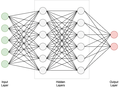
It's called a neural network. And the thing called Universal Approximation Theorem mathematically proves that a neural network can solve any problem to any accuracy level if you just find the right set of weights. A typical neural network usually consists of multiple layers, as shown below.
And the amount of hidden layers determines how deep the network is, right? So, we can think about machine learning for neural networks as deep learning. There are proper classifications of those terms in the literature, but sometimes using intuitive explanations are easier to understand and remember.
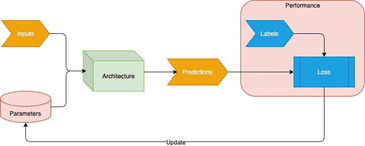
Nowadays, we don't use the same terminology as in the Arthur Samuel version of machine learning, but we use the same idea.
- We still have inputs which are samples for our task (e.g. images of smiling faces)
- Weights are called parameters.
- Model is called architecture. And it's simply a function for which we adjust the weights to get it to do something. It could be a neural network function such as ResNet, AlexNet, just to name a few.
- Instead of results, we have predictions.
- The labels are the target result for the given input sample. For instance, the label could be the input image classification - is it a cat or dog, what kind of vehicle, coordinates of the object on the image, etc.
- The measure of Performance from Arthur Samuel's version is known as the loss calculated from labels and
predictions.
The loss is a function that evaluates how well specific algorithm models the given data, e.g. how close the prediction is to the target label. Suppose predictions are far away from the expected result. The loss function would result in a large number next used to update parameters accordingly to reduce the prediction error. Several loss functions might be used that depends on the model's application. I'm going to touch on that subject in one of the follow-up articles. - Architecture, together with parameters, is called a model nowadays. So whenever you see the term "model", it means it is a specific architecture (neural network function) together with the trained parameters.
Based on what we've learned so far about machine learning, we can conclude with a couple of fundamental limitations we must never forget:
- You need data to train a model - a model must be fed with examples of your data to learn from. And it also means that a model can only learn from patterns seen in the input data. It can't give you the correct answers on data pattern it never saw (e.g. if you trained a model with cars pictures, it can't predict people faces, or if you trained the model with people faces, it would not be able to properly work with manga characters).
- Data examples are not enough. As I explained above, labels are needed to calculate the loss so the model's parameters could be adjusted to let the model learn something.
- A trained model always creates predictions, not actions. So it determines how you can potentially use it in your application.
Equipped with that basic knowledge, let's jump directly into the code and see deep learning in action.
Let's build and train a state-of-the-art model
We will not build any neural network from scratch nor implement the learning loop from scratch. Instead, we will use what's available in libraries, to create a practical machine learning application ready to use in production. We will make a smiling faces detector achieving near-perfect accuracy with some room for improvements that I can show you in future articles.
We will be using the FastAI library that is based on the PyTorch. The latter is the most used by researchers nowadays, but it's not friendly for beginners in the field. FastAI, on the other hand, provides higher-level APIs on top of PyTorch that simplifies and speeds up coding, at the same time giving the ability to use low-level PyTorch capabilities. All the code I present here is developed using Jupyter Notbook running on Paperspace cloud platform, specifically Paperspace Gradinet where you get access to a Juptyer Notebook instance backed by a free GPU.
I shared my Paperspace Gradient notebook with all the code presented in this post, so you can create an account for free and spin off your own instance with Free GPU to try the code by yourself.
To build our image classifier, we need to train a model with some data. We will be using
Large-scale CelebFaces Attributes (CelebA) Dataset that contains
over 200k celebrity images, each with 40 attribute annotations. The dataset can be employed for various computer vision
tasks such as face attribute recognition, face detection, landmark localization, and face editing & synthesis. For the
sake of this article, we will be using only 20k images and will rely on a single attribute, which is Smiling.
The code below is the full implementation. It simply gets a list of 20k files together with the Smiling attribute and
then runs the training loop that tries to learn which images are smiling faces and which ones are not.
import pandas as pd
from fastai.vision.all import *

celeb_img_dir = '/datasets/celebA'
celeb_attrs = 'https://raw.githubusercontent.com/togheppi/cDCGAN/master/list_attr_celeba.csv'

data_frame = pd.read_csv(celeb_attrs)[['File_name','Smiling']].sample(20000)
data_loaders = ImageDataLoaders.from_df(
    data_frame,
    celeb_img_dir,
    valid_pct=0.2,
    seed=42,
    label_col='Smiling',
    item_tfms=Resize(224))

learn = cnn_learner(
            data_loaders,
            resnet34,
            metrics=error_rate,
            pretrained=True)

learn.fine_tune(2)
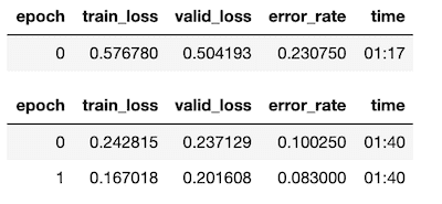
After about 3 minutes, we can see an error rate of around 8%. And the error rate is our performance metric that measures our model's quality - it merely tells a proportion of incorrectly identified images after the training process. I will explain every line of the code in detail in a moment, but now let's try our model. Thanks to the Jupyter notebook, we can quickly build a simple application that simulates potential production usage. It is an essential takeaway to do the end-to-end application from the start. That way, you will learn something new from each iteration instead of spending lots of time preparing an ideal dataset, thinking about improvements, or simply planning all the steps.
Here's the code that creates a UI widget where you can upload an image and classify it using our model.
def _on_upload(change):
    widget = change['owner']
    img = PILImage.create(widget.data[0])
    show_image(img)
    predict(img)

def decision(prob):
    if prob >= 0.9:
        return "Definitely smiling face"
    elif 0.9 > prob > 0.5:
        return "I'm quite sure it's a smiling face"
    else:
        return "In my opinion this person is not smiling"

def predict(img):
    _, _, probs = learn.predict(img)
    print(f"{decision(probs[1].item())}. Probability it's a smiling face is {probs[1].item()*100:.2f}%")


label = widgets.Label("Welcome to smiling faces detector. Upload your images below")
uploader = widgets.FileUpload(multiple=False)
uploader.observe(_on_upload, names='data')
widgets.VBox([label, uploader])
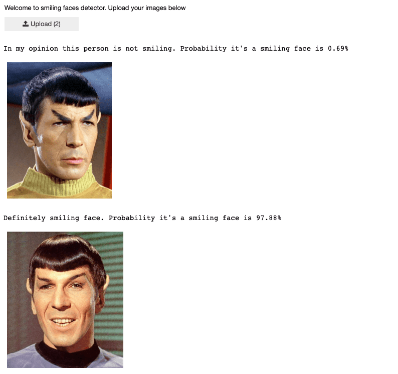
Once executed, we can interact with the widget and upload images to see how our "Smiling faces detector" application works. As you can see, we're not using the model's result as our decision directly since it's just a prediction. Instead, the application checks if the "smiling face" probability is big enough to get back a final decision.
Results look great. Apparently, it's capable of detecting Vulcan smiling faces, probably because Spock is a half-human. If you tried the application with images containing pictures of people but not images cropped around the face, you'd probably end up with false results. As I mentioned initially, our model never saw such images during the training - the dataset we used actually contains just human faces.
You might be wondering if our detector would be useless in real-world pictures when you seldom have people photos cropped to the face only. And you would be right. That would require a more complex approach where we have either two models or one model that aggregate two tasks. First, it would need to locate people faces on the picture (object detection and/or localization). The result of that localization would give us a boundary box of the face location. Then the fragment of the image, described by the boundary box, could be a subject of the classification model that makes a final decision.
So, we trained our classification model and did a PoC of the actual application. You know now, we're using a neural network, and we're doing machine learning, and you know what machine learning means. Let me explain now what we actually did.
Code deep-dive
Let's look at the code again.
import pandas as pd               (1)
from fastai.vision.all import *

celeb_img_dir = '/datasets/celebA'
celeb_attrs = 'https://raw.githubusercontent.com/togheppi/cDCGAN/master/list_attr_celeba.csv'

data_frame = pd.read_csv(celeb_attrs)[['File_name','Smiling']].sample(20000) (2)
data_loaders = ImageDataLoaders.from_df(  (3)
    data_frame,                           (4)
    celeb_img_dir,                        (5)
    valid_pct=0.2,                        (6)
    seed=42,                              (7)
    label_col='Smiling',                  (8)
item_tfms=Resize(224)) (9)- First, we need to import the required libraries. We're importing the most famous library in data science called
Pandas library that helps us work with tabular data. We're loading it as
pdnamespace. Then importing FastAI library that provides all it's necessary to perform any computer vision task. - Here, using Pandas library, we're loading the CSV file that contains a mapping between the file name and the face
attributes. Then we're telling to pick only two columns (file name and smiling attribute), and we take random 20k
rows as a
Dataframeobject. Here are a couple of sample records from our data frame to help you understand its outcome.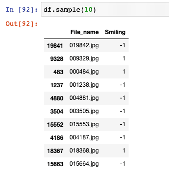
- Here, we're creating a FastAI data structure called
Dataloader. This structure organizes our data in the form required by the learning process. We useImageDataLoadersfactory class as we're about to load images. Factory methodfrom_dftells that we're about to load data described by the Pandas data frame. - It is our data frame object we created before.
- A root path where image binaries are available on the server.
- Defines a validation percentage. We're telling here to grab randomly 20% of our data that will not be used for training. And this data, called validation data, will be used to calculate our metric (error rate) to see how good our model is after the training. Validation data is a critical aspect of deep learning, so we come back to this topic later in this article.
- It just initializes the random numbers generator.
- We're telling here that the
Smilingcolumn from our data frame provides a label for a given image. - It tells the data loader to resize each of the images to 224x224 pixels as we need to provide our model images with the exact dimensions. The reason why we're doing it is that the training dataset might have images of different sizes. Additionally, to achieve the best computation performance, data is loaded into GPU in batches as a single multidimensional matrix. If you think about the 3D matrix, each layer must have the same dimension, and each one represents a single image. And that imposes to have images of the same dimensions. Why 224 pixels? It's a compromise between training speed, available GPU memory and impact on the model accuracy. You can pick bigger sizes, but the training time would increase, or you'd need to use smaller batches due to the lack of GPU memory (or even you'd need more GPU memory). The 224x224 is widely used by researchers, so I did use it too. I'll explain more about batches, how things are calculated in another article.
Up to this point, we just created Dataloaders obect that actually doesn't load anything yet, but creates a lazy
iterator having an API providing two-stream of the data: training data and validation data. And image resizing will
happen once the training loop starts reading the data. A data loader doesn't provide each item one by one as it would be
very ineffective. Instead, it processes images and provides the training loop in batches. Thanks to that, the underlying
PyTorch library can leverage the GPU's full power and load and calculate data for the whole batch at once.
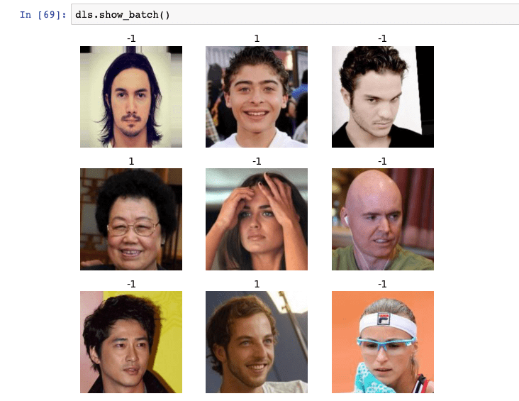
Once Dataloaders object iscreated, we can inspect it to see what's inside by sampling a random batch. Images annotated
with 1 are smiling faces.
In the remaining part of the code, we're creating a learner object that is, as the names suggest, the thing that does
the training.
learn = cnn_learner(
            data_loaders,                 (1)
            resnet34,                     (2)
            metrics=error_rate,           (3)
            pretrained=True)              (4)

learn.fine_tune(2)                        (5)
We're using a cnn_learner here that creates a learner for Convolutional Neural Network. CNN is the current
state-of-the-art approach for computer vision inspired by how the human vision system works. There are many different
architectures of such networks, but here we're about to use ResNet that is both accurate and fast for many problems.
What CNN architecture to pick? Practice shows that it is not a critical part of the process, and most practitioners don't spend much time on it. It's usually based on experience or running experiments to determine which one is better for a given task.
- Our data loaders object we created before.
- Neural network architecture we chose, in this case, ResNet34.
- This parameter pecifies what metric to print out after the training. And the metric is always going to be applied to the validation dataset. That's what you are always going to do, checking performance on data your model hasn't seen during the training.
- It says learner object to set the weights of the model to values that have already been trained by experts. Pretrained models are used by the Transfer Learning method, and I will describe the concept later in this article.
- Finally, we're calling a method on our learner that starts the training process. The number
2is the number of epochs - it tells the learner how many times to look at each image. The number of epochs is an arbitrarily chosen value that depends on the available time or how many times you found it gives the best accuracy. The good thing is that you can always rerun the learner again, observe results, and then pick your optimal number. For the sake of this article I used two epochs as I found it just enough to achieve acceptable accuracy.
Validation data
I mentioned before that we're putting aside some part of our data so that the process can use it for validation purpose. Why do we need to do this?
When training a model for enough long time, it will eventually start memorizing the label for each image instead of learning the features from the pictures that lead to the given prediction, which is called over-fitting. Such a model could start cheating you as if you tried it with the data you used for training, it would give you perfect results. But this is not your intention. You want your model to learn something from the examples to classify new data when they come. And the only way to assure you're doing it right is to have a validation dataset - the data you will not show to the model during the training. In our example, we used the FastAI feature to prepare such validation set automatically by picking randomly 20% of images for validation purposes. The remaining 80% were used for the training only. Of course, it doesn't mean you need to do it all the time. You might have a dataset already providing training and validation data sets.
In fact, it's not the whole story. In the real-world, a model is not being trained once. You often need to modify some bits in the model or the training routines, e.g. some optimizations in the layers, trying different architecture, learning rates, data augmentation, and many more; these are called hyperparameters. After all of those efforts, you will start seeing your model is getting better and better, as your metric tells. But it might be the case that it actually starts fitting to the validations set.
Machine learning practitioners take a more rigorous path and prepare a third data set, called test data set. And this data set becomes something they must hold back even from themselves until the end of the project when all optimizations have done. Then you could evaluate your model against the test dataset.
It's even more critical if you're looking at vendors offering AI services, and you see they are presenting outstanding results. A good practice is to always verify it. So, put aside some of your data and never show it to the vendor. Once modelling is done, use it to verify results. Only then you will be assured about the actual performance.
So, the rule of thumb is:
- Always put aside some of the data to create a validation set (either manually or automatically)
- Do not show this data to the model during the training and only validate your model after each epoch of the training.
- If possible, create a third data set used to evaluate the final result of your project. And never ever use it during all your efforts during the project.
Ok, you have data but not the validation set. So, you picked the route I showed here and simply randomly picked some percentage of it as validation data. There is bad news, depending on the task, it is not so simple and could lead you to the wrong results. First, you need to understand the nature of the data and the task you are working on as preparing either training or validation data is always a process that requires human judgment. Let's look at two examples mentioned in the Fast.AI course to give you some idea of what it means. These are great representatives of real-life problems and how to deal with them.
Time series data
If you're working on a model that predicts future data based on past events (e.g. weather conditions, stock prices, etc.) and you have raw data as shown in the first picture, how would you split it? If you split it randomly like shown in the middle, your model would do a great job filling those gaps but terrible predicting future points. In that case, all you need to do is to use earlier data as your training data and later data as validation data.
Image data
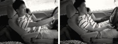
With image data, it might require much more thinking and understanding of the task nature. A great example of this comes from the Distracted driver Kaggle competition, where inputs are the pictures of drivers at the wheel of a car and labels are categories such as texting, eating or safely looking ahead.
Suppose you used one of the images shown below in your training set and the second one in the validation set. In that case, the model might be performing great on pictures of that person, but not necessarily if tested with different persons' images.
However, if both photos were used in the training set, a model may be overfitting to this specific person's particularities and not just learning the states.
The solution would be to build a training and validation set to have photos of different people across all states and assure the validation data contains unique people. Only that way, you will be assured that the model learned states, not the person particularities.
Transfer Learning
If you remember the code, I said we use the pre-trained model (see pretrained=True parameter of the learner). As the
name suggests is the model that was already trained before by someone else. And there is a technique called Transfer
Learning which enables us to use pre-trained models. Why did we do that, and what are the benefits?
In fact, this is a technique you should use most of the time. And there are a couple of reasons behind it. First of all, it's a huge time & cost saver. Training the model from scratch would require an enormous amount of data, so the time and cost. E.g. Resnet34 trained with ImageNet with as around 1.3Millions of images (160GB of data) can take weeks of training with an affordable price GPU unit, not to mention the time spent on tunning the training process or the model etc.
So in our case, we used a pre-trained model that was already capable of understanding some concepts on the images, so we don't need to have many training images. As you can see, the single epoch of the training lasts about 1 minute instead of hours. Even if we optimized certain bits and pieces and run much more epochs, it would be still far away from weeks of training.
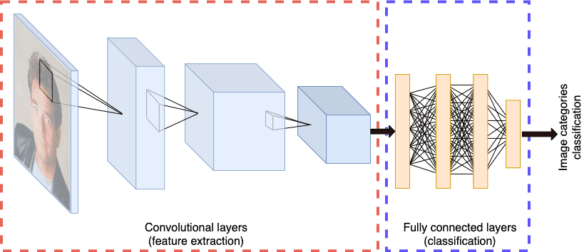
Before explaining how and why transfer learning works, let me quickly explain CNN architecture first. In the below diagram, I showed the typical CNN architecture containing two types of layers. Convolutional layers and fully connected layers. The real architectures are a little bit more complex as they have more layers, and there are multiple intermediate optimizations steps, but it's not relevant at this moment.
As the name suggests, convolutional layers are the core building blocks of any Convolutional Neural Network (CNN). Convolution is a well-known computer vision technique for tasks like finding edges in the image or applying filters to sharpen or blur the image and transform it to get the edges only.
After convolutional layers, we have a different structure called fully connected layers. These are the layers of neural networks we all know. Those layers actually perform final decisions specific to our task, such as classification, object detection and so on.
Why it's done in such a way? Let me explain it step by step.
Convolutional layers
When the image is convoluted with the first layer's filter, we will get a much smaller picture with stressed-out simple structures like edges, lines, gradients. In the subsequent layers, convolutions are done on results from previous layers to extract more complex concepts from the image. Finally, in the last layer, we have convolutions results representing the image's most complex abstract concepts. It could be things that we as a humans interpret as a piece of text, car wheels, cell phones or something else. Of course, it is just an oversimplification.
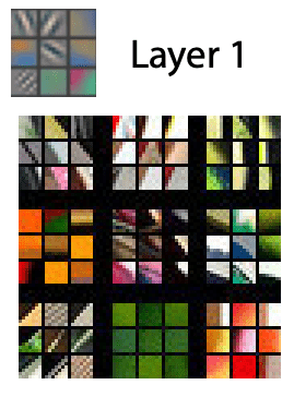
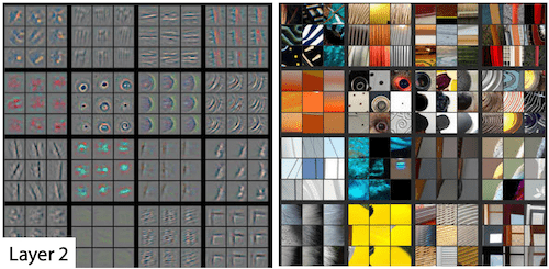
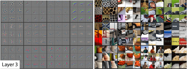
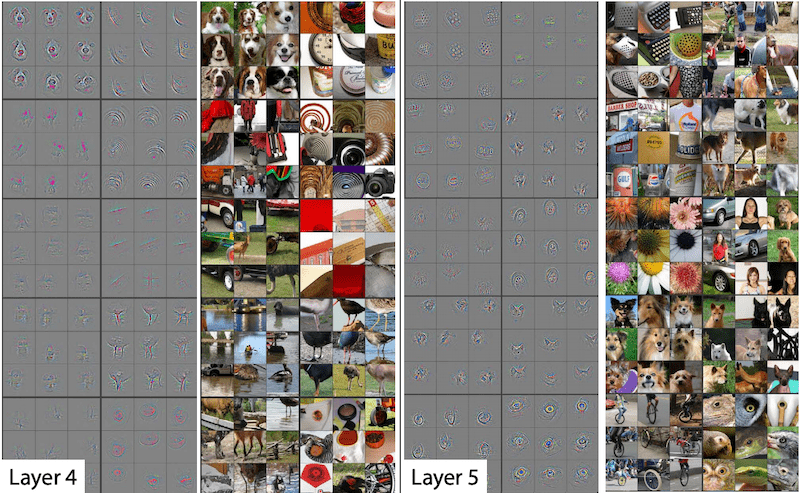
Recent studies show this is the right way of thinking. The best example of that is the paper "Visualizing and Understanding Convolutional Networks" which shows how to visualize the neural network weights learned in each layer of the model. The studied model was based on AlexNet architecture with just 5 layers, which is much smaller than what we used in this article, but it applies to any CNN architecture.
Here are a couple of visualizations from the paper. For each layer, the image part with the light grey background shows the weights reconstructed into a pictures and on the right-hand side shows the image patches from the training set that most strongly matched each set of weights.
So, the first layer activates mainly on simple concepts like diagonals, horizontals, and gradients.
On layer 2, we see more complex structures like corners, circles, repeating patterns.
On layer 3, we can see some semantic components, like car wheels, text or some diagonal structures.
On the last layer, we see it captures the visual structures most likely to be pets, human faces, text labels, flowers, etc.
It was just 5 layers network; imagine what rich features ResNet with 34 layers can extract from the images.
This and other studies show that those convolutional layers capture abstract features about the images. Then we can get those weights from the already trained model and use them for other purposes by just adopting the head layers (fully connected layers).
Fully connected layers
As I mentioned before, the Universal Approximation Theorem proves that neural network structure can solve nearly any problem given the proper weights were found. So, why we can't just use such a network instead of doing convolution things. There are multiple reasons like computation stability, but the most important reason is that it would require massive computing power. Even for relatively small input images, we could end up with tens of millions of parameters just on the first layers, so at the end of the day, we could end up with a network requiring a few of 100M of parameters to train. As a comparison, our ResNet34 network contains around 20 million parameters for all 34 layers. So, CNN architecture can be seen as neural network optimization.
Thus, we know that convolutional layers extract features. The fully connected layers can now solve any task (see Universal Approximation Theorem) we want using those features instead of relying on each pixel. It could be image classification as in our model or object detection, or even generation of new images.
Transfer learning method
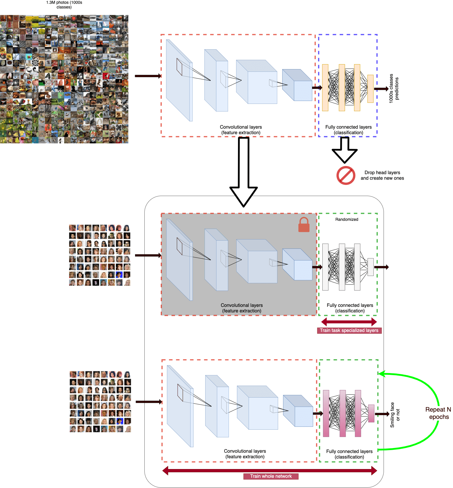
We learned about how the CNN extracts features from the image and why we have fully-connected layers. Let see how the transfer learning process looks like in general. If you look at the diagram below, the first row shows that CNN architecture is trained using the ImageNet dataset having around 1.3 million photos and about 1000s categories of images. Such a model is capable of classifying the given image within those 1000s categories.
The procedure can follow these steps:
- Take a body of the pre-trained model (convolutional network with all the trained parameters)
- Get rid of original fully-connected layers (called the head), as they were specialized to the original task - which was classification on 1000s categories.
- Replace that head with a new set of fully-connected layers with the structure tailored to our task (e.g. smiling or not faces, instead of 1000 categories)
- Using our task-specific dataset, train the model but only the head layers (task specialized fully-connected layers)
- Then unlock the pre-trained body and, this time, train the whole model (fine-tune) for N number of epochs.
All of this is implemented already by FastAI, so you don't need to reinvent the wheel. There are also lots of modern optimizations done inside, but it is a subject for other articles.
This technique gives us a couple of benefits such as we don't need to have a massive data set and still getting great performance results. And with less data, we also save time and the overall cost of building the model.
You might be wondering where I can get those pre-trained models. There are a vast amount of resources on the internet, just to name a few:
- PyTorch itself provides the most famous models ready to use].
- FastAI itself provides PyTorch models as well as a couple of extras
- There is a great resource called Model Zoo, where you can find any type of pre-trained models not only for computer vision tasks but also Natural Language Processing (NLP) and others
- If you're interested specifically in NLP, the best resource is the The Huggingface
I also found quite interesting Google's recent contribution to the AI community. At the end of 2019, their research team published a paper Computer Vision Model Big Transfer, when they attempted to meet the goal of training an ultimate computer vision model. A model trained with a giant database of labelled images to achieve a state when such a model could be used for any other smaller tasks, like the starting point for every computer vision problem (thanks to transfer learning). They trained three models (all models are just standard ResNet architectures) with a different set of data:
- BiT-S - a small one trained with simply well-known ImageNet containing 1.3M images
- BiT-M - a one trained with ImageNet21k dataset containing 14 million images
- BiT-L - is the most impressive one, trained with a dataset of 300 million images. There are not many images on the internet that were not used in this dataset.
The two smallest ones (S & M) are released and available to the community. The biggest one is not available. I think it's due to the cost involved to train the model. The paper vaguely presents some figures on time spent as 8 GPU weeks vs 8 GPU months, and it might be an indication of time and resources involved in the training process.
Summary
Even though this post is quite long, I feel like I just scratched the surface. It seems to me that I will keep continuing with this subject as there are much more exciting areas to study or try, such as:
- Building a web service running our model and/or using AWS/Azure or Google services to train and run models - so more of an end-to-end project
- More techniques, tricks & methods to improve model overall performance
- Finally, Natural Language Processing, Tabular data, Recommendations or GAN networks (networks capable of generating new data)
I hope you enjoyed it and learned something. If you'd like to learn more about using deep learning in practice, think about the small project and start building it. If you feel overwhelmed and don't know where to start, I encourage you to start Fast.AI online course course (100% free) when you can efficiently learn a deep learning craft.
Hero image by Philipp Marquetand from Pixabay, opens in a new window
Featured image by Philipp Marquetand from Pixabay, opens in a new window

