The demand for machine learning has been growing constantly over the years. Despite more and more people getting interested in this field, the supply of experts seems to still be lagging behind. In this blogpost, we'll use H2O's AutoML to create a highly-performant machine learning model with no math or domain knowledge required.
Machine learning is thought by many to be too arcane a topic to pick up without spending years to study the math behind it. However, creating custom machine learning models doesn't need to be too demanding. Most often, developers can look into numerous existing machine learning libraries or frameworks, and put to use some tried and tested methods developed by experts over the years. With correct tools, you don't need to know much about the intricacies of machine learning to create an effective model. Some libraries go as far as to automate the whole process of model creation, reducing the user's responsibility to supplying a dataset and defining the desired output.
H2O
H2O is an open-source, distributed platform designed to make it easy for non-experts to experiment with machine learning. It provides a convenient interface for numerous machine learning models, such as artificial neural networks, decision trees, linear models, and much more. By sharing a simple common interface, these models are easy to train and use interchangeably according to your needs. At the same time, H2O authors leave a lot of flexibility in the models' APIs. The number of parameters one can configure for each model seems overwhelming at first. However, you can always go with the defaults, which very often turn out to be just fine. All in all, the design of the tool makes the learning curve very gentle. You don't have to know any theory to start working and the interface still allows for a high degree of customisation, so you can always try to fine-tune your model if you feel like it.
Throughout this tutorial, we'll use H2O 3.32.0.3 with Python 3.6.10.
AutoML
Automated machine learning, often simply called AutoML, is a broad term encompassing various techniques of automating the process of training ML models. AutoML makes machine learning much more accessible by reducing the volume of knowledge one has to possess to start experimenting in this field. Additionally, even if you know a fair amount of machine learning theory, AutoML can still prove useful by automating some menial task for you, such as searching for optimal model hyperparameters. There are numerous steps of a machine learning pipeline that can be automated, for instance:
- Data preparation
- Feature engineering
- Model selection
- Hyperparameter optimization
- And more
Each category of AutoML comes with its own challenges. In this blogpost, we'll focus on H2O's implementation of AutoML, which automates model selection and hyperparameter tuning.
Let's see this all in action
Enough with the theory, let's test the AutoML capabilities on a real dataset. To show the power of H2O's AutoML, we'll use a public database uploaded to kaggle.com called Titanic. The dataset contains information about Titanic passengers, including, but not limited to:
- Ticket class
- Sex
- Age
- Number of siblings/spouses aboard the Titanic
- Ticket number
The complete list of attributes can be found in the description of the dataset. It's worth mentioning that the attributes have diverse types - some of them, for instance, the ticket class, take one value from a limited list of possible options (first, second, or third class), while others, for example, age, are numerical.
The target variable, which is a variable we would like to predict using a machine learning model, is called Survived
and takes 1 if the passenger survived and 0 otherwise.
Loading the data
The first step in our workflow is loading the data into an H2O's tabular structure called H2OFrame. If you are familiar with pandas, you should feel comfortable using H2OFrames, as they're very similar to DataFrames.
To load the data, you first have to download it (link) in a
CSV format. There are two files present - test.csv and train.csv. For our purposes, we'll use train.csv only. The
other one, test.csv, is missing the target value and is used if you want to upload the results of your model to
kaggle.com to compare your solution with others'. The training dataset is the one we'll use
to gauge our solution ourselves by dividing it further into two sets - one we'll use to train the model, the other to
test its performance.
Okay, let's dive into the code. Before doing anything, let's import h2o and initialize it.
import h2o
from h2o.automl import H2OAutoML
from h2o.estimators import H2ODeepLearningEstimator
from h2o.explanation import explain
h2o.init()
Now, we can load the CSV file we've downloaded earlier and peek inside. After loading the data, we want to tell H2O to
treat this as a classification problem (predicting either 0 or 1) instead of a regression task (predicting a real
number, for example 0.12) by using a built-in asfactor() function.
data = h2o.import_file('train.csv')
data["Survived"] = data["Survived"].asfactor()
data.show()
First ten entries in the dataset are displayed, so we can verify that everything has loaded properly.
Now, we'll choose which columns will be used as predictors and which one as a target variable. For predictors, we'll use
all the columns apart from the ones that are unique for each passenger (PassengerId and Name in this case), and the
one storing the target variable (Survived). The column names will later be passed to the model, so it knows which
columns to use for training and which is the one we wish to predict.
target = "Survived"
predictors = data.columns
for col in ["PassengerId", "Name", target]: predictors.remove(col)
Let's take 80% of the data for training purposes and leave the rest as a test set which will be used to gauge the
model's accuracy on unseen data. The split is random by default, but, for educational purposes, we'd like to get
reproducible results every time we run the code. To this end, we'll pass a constant value to the seed argument.
Throughout this post, we'll do the same for every function with randomness in its implementation.
train, test = data.split_frame(ratios = [0.8], seed=1234)In this tutorial, we'll skip any further data preprocessing to keep the solution as simple as possible. Normally, however, the next steps would include cleaning up the data, feature selection (choosing which columns are meaningful and should be left for training), feature extraction (creating new attributes based on the old ones), and more.
For the sake of simplicity, we'll skip this for now and go straight to business. As the dataset is relatively well-structured, the lack of preprocessing shouldn't prevent us from getting meaningful results. Additionally, we don't have to do any data conversion, such as one-hot encoding of the categorical attributes, since H2O will do this for us under the hood.
With the data ready, you should now pick an ML model you'd like to use. There are many options to choose from, for instance:
- Neural networks
- Decision trees
- Linear models
- Naive Bayes classifiers
The choice of a model is a fundamental decision in the whole process, and often has the biggest impact on the performance of the end solution. It also dictates many other decisions, for instance, the way you can tweak model parameters. Furthermore, various models differ in things like training time, the amount of resources needed, explainability, and more.
After choosing a model, the next step is the implementation phase. The amount of expert knowledge you have to possess depends heavily on the library or framework you settle for. Some frameworks make it easier than others to create custom models. For instance, if you want to implement a neural network, you may do it with no libraries at all (dust off your algebra textbooks, then), you can use Tensorflow 1.X if you want to have some things automated for you, or frameworks like Keras if you want to make the process even simpler. Even though they make model creation more convenient, such frameworks often still require some knowledge about the theory behind machine learning.
Choosing a model ourselves
Having loaded the data, we can use H2O's interface to train one of the models available. However, without any domain knowledge, we often don't know which model has the highest chance of performing well. Additionally, it'd be hard to tune its parameters without knowing their meaning.
Let's not worry too much and choose any model, so we can compare it to the one found by AutoML later. Nowadays, neural
networks seem to get the most hype, so let's pick a neural network as our model. In H2O, neural networks are accessible
under the H2ODeepLearningEstimator type. To train the default version of the estimator, it's sufficient to pass the
train and test set to it and specify the predictor and target columns.
nn_model = H2ODeepLearningEstimator(seed=1234, reproducible=True)
nn_model.train(x=predictors, y=target, training_frame=train, validation_frame=test)
After some time, the model is trained. Let's check its accuracy measured on the test set.
accuracy = nn_model.model_performance(test).accuracy()
# The accuracy has [[threshold, max_accuracy]] format, printing only the actual accuracy:
print(f"Accuracy: {round(accuracy[0][1]*100, 2)}%")
Output:
Accuracy: 83.24%Not too bad, the accuracy is slightly higher than 83%, meaning the model is wrong roughly once every 6 predictions. Are we sure this is the best we can do, though? We went with the default arguments, so it's reasonable to expect that by tampering with the model a bit we could make it perform even better. One way of improving the predictions is to tweak the model parameters, for example, the number of hidden layers in the network, the number of epochs to train for, the learning rate, and more. The search for optimal parameters can be effective but is often time-consuming, and the impact of some parameters is not always predictable.
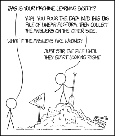 Credits: xkcd
Let's see how we can take the burden of choosing and tuning ML models off our shoulders by using the H2O's AutoML functionality.
Finding the best model using AutoML
First, we have to take a step back. We have our data loaded, but have no idea which model to choose and how to optimize it. Fortunately, we can delegate the job of finding the best model (and its parameters) to the AutoML tool.
The way we do the training is very similar to the one described above. In this case, we tell H2O to train 20 different models. We'll then check the performance of the best one and see whether the automated solution is superior to the model we've trained previously.
aml = H2OAutoML(max_models=20, seed=1234)
aml.train(x=predictors, y=target, training_frame=train)
Note, however, that we don't pass the test set to the training function. This is because, by default, AutoML will use cross-validation on the training set to gauge the performance of the models and, additionally, train a stacked ensemble model. To keep it simple, we'll leave it this way. We'll use the test set later, in order to compare the model created by AutoML with the one we've trained ourselves.
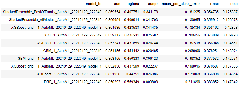
The output of the AutoML training is a leaderboard - a table storing information about all the models trained throughout the process. Each row includes a model identifier as well as various performance metrics.
lb = aml.leaderboard
lb.head()
The top-performing model is called a leader. In this case, two best models are stacked ensembles, which are a special kind of ML models combining a collection of other models in order to provide better predictions than any of the constituent models separately. You can read more about the concept behind stacked ensembles here.
Let's access the leader model directly and test its performance on our test set.
leader = aml.leader
accuracy = leader.model_performance(test).accuracy()
print(f"Accuracy: {round(accuracy[0][1]*100, 2)}%")
Output:
Accuracy: 87.15%Not too bad! We can see a pretty significant accuracy improvement compared to the deep learning model we've tested previously (87.15% vs 83.24%), all without concerning ourselves with model selection or parameter tuning.
Bonus: Explainable AI
The popularisation of implementing AI-based solution to tackle real-world problems has led to a need for models capable of producing some sort of explanation of their outputs. For instance, a machine learning model predicting one's credit score without giving any insight into the reasoning behind the decision is considered by many to be unacceptable. Without knowing the model's "thought process", it's impossible, for instance, to ensure that the model doesn't discriminate against certain groups of people. Furthermore, such a model doesn't give any feedback on how to influence the response by modifying the input data. Techniques implemented to provide human-understandable responses of AI systems are often jointly called Explainable AI (XAI).
Fortunately, H2O comes with an explainability module out of the box. You can read the documentation describing this feature here. Getting a detailed explanation of our best model's outputs is as simple as calling:
explain(leader, test)Unfortunately, some features like variable importance are not available for stacked ensembles yet, so, to see the explainability report in its full glory, let's investigate the best model which is not a stacked ensemble:
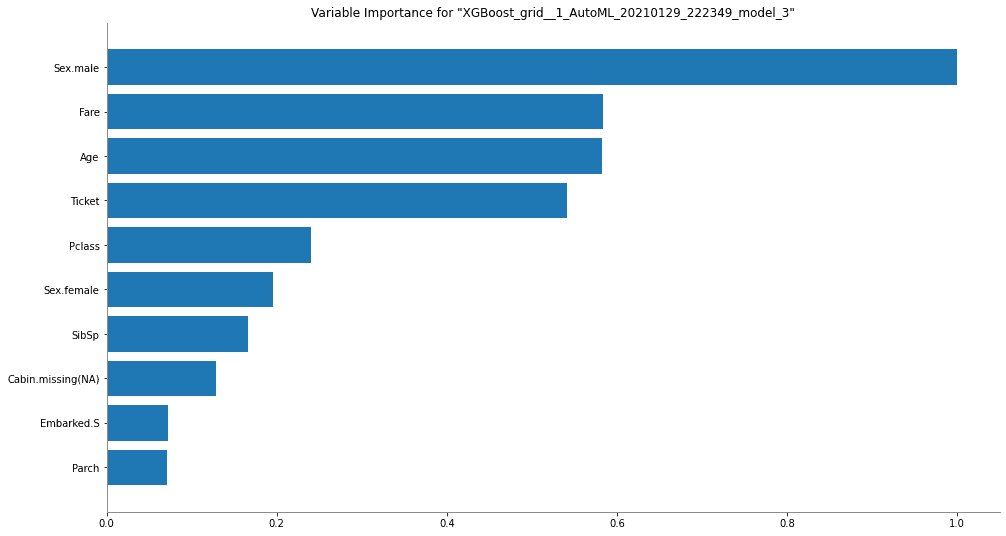
explain(h2o.get_model('XGBoost_grid__1_AutoML_20210129_222349_model_3'), test)The report shows multiple features of the selected model, for instance, the variable importance chart:
We can see that the most important attribute in the dataset is the sex of the passenger (which was divided by H2O into
two binary variables - Sex.male and Sex.female).
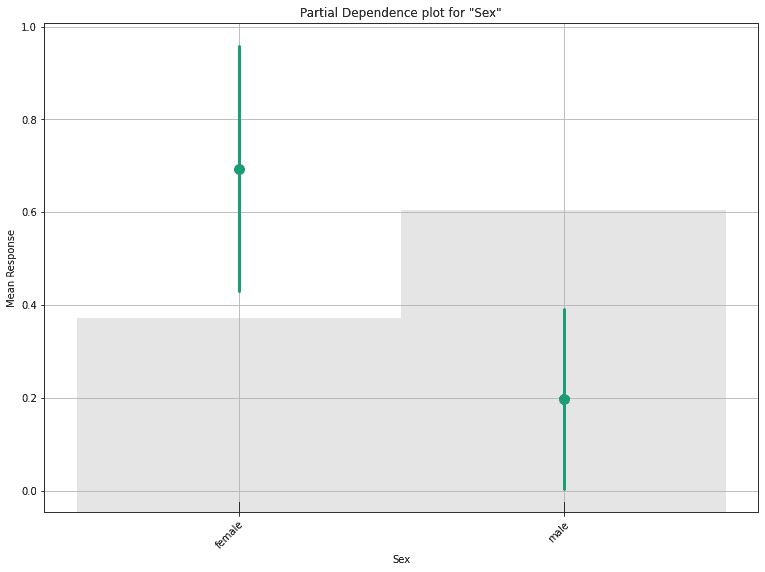
Now, let's look at the partial dependence plot for this attribute. Such a plot shows the expected response of the model as a function of a selected input variable. We can see that the model predicts higher chances of survival for females:
The bars show the distribution of the variable, we can see that there were more males than females on the board.
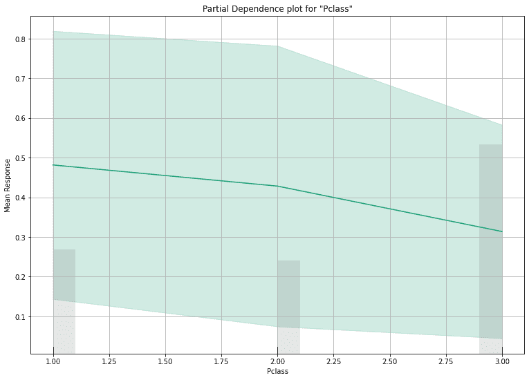
Let's look at one more partial dependence plot, this time for the ticket class:
As can be seen, the higher the class (first being the highest), the higher the chances of survival.
The information provided by the explainability module doesn't end there, as there are more metrics contained in the summary, such as SHAP values. I encourage you to dive into the report yourself, you may be surprised by what you find.
If you want to see the full Jupyter Notebook containing the code from this blogpost, you can check it here.
Summary
In recent years, the significance of machine learning solutions has become even more evident. An ever-growing number of businesses incorporate ML into their working pipelines or the products they offer. Tools such as H2O's AutoML show that it's possible to jump on the ML bandwagon without high costs. Being a turnkey solution, AutoML doesn't promise to be the optimal solution at all times, but keeping in mind the great benefits it can bring for little effort - it's definitely worth looking into.

