A guide to model calibration

When working with machine learning classifiers, it might be desirable to have the model predict probabilities of data belonging to each possible class instead of crude class labels. Gaining access to probabilities is useful for a richer interpretation of the responses, analyzing the model shortcomings, or presenting the uncertainty to the end-users. Unfortunately, not all machine learning models are capable of producing responses that can be directly interpreted as probabilities backed by the data. In order for this to happen, the model has to be calibrated. In this blog post, we'll introduce the theory behind machine learning model calibration, explain the methods used in calibration, and implement a simple framework for calibrating any classifiers, regardless of their implementation details.

Classification remains one of the most popular tasks in machine learning, be it fraud detection, sentiment analysis, classifying images or others. Technically speaking, the goal of classification is to assign labels to data samples. It comes in different flavours, the easiest one being a binary classification, in which the input is classified as coming from one of just two classes. A bit more challenging alternatives are multi-class (one target class, more than two possible classes) or multi-label (multiple targets) classification. The possibilities don't end here, as, for instance for computer vision, there is also classification with localization, object detection, and image/instance segmentation. All the aforementioned cases have one thing in common - the algorithm produces a discrete response - the possible outputs are limited by the number of categories represented in the dataset.

Different models, different outputs

In some cases, the fact that a model has only a limited number of possible outputs is somewhat natural. For example, with basic decision trees, going down the tree narrows down the space of possible responses until a leaf with a single class is reached. The simplest trees can do this by dissecting the space of possibilities in such a way as to minimize the total entropy. Nowhere in the process is it necessary for the model to use numbers instead of labels to represent the final outcome.

Other methods, such as classical neural networks, are purely numerical. The input tensor is forwarded through network layers, with multiple nonlinear transformations along the way, yielding an output tensor of real numbers at the end. In the case of binary classification, it can be a single number. In multi-class problems, it's a vector of the length equal to the number of classes.

With models like these, the numerical output has to be transformed into the final output. Usually, with multiple labels, it's enough to look at the category with the highest value assigned, and choose it as the final class. This works perfectly well, but you might feel tempted to use the exact numerical information as the confidence of the model, i.e. the probability it assigns to the input belonging to the predicted class. This is where things can get complicated. You can't really take it for granted that the number underlying the classification is meaningful as the model confidence (e.g. the model is not necessarily twice as confident when returning 0.8 compared to 0.4). If you want to interpret the number as a probability score, you have to make sure that the model is calibrated.

Calibrated model

A machine learning model is calibrated if it produces calibrated probabilities. More specifically, probabilities are calibrated where a prediction of a class with confidence p is correct 100*p percent of the time. Consider this example: if a model trained to classify images as either containing a cat or not, is presented with 10 pictures, and outputs the probability of there being a cat as 0.6 (or 60%) for every image, we expect 6 cat images to be present in the set. With calibrated probabilities, we might directly interpret the produced numbers as the confidence of the model. When encountering easy samples from the dataset, for which the model is rarely wrong, we expect the model to produce values close to 1. For harder ones, we expect the number to be lower, reflecting the proportion of misclassified examples in such sets.

As another example, imagine two models trained to predict the probability of a coin toss resulting in heads. We assume that the coin is fair and each toss yields a truly random result. In this scenario, no model should achieve accuracy other than 50% (unless the model is capable of predicting the future, that is). One of the models outputs 0.5 (or 50%) each time, while the other alternates its predictions by outputting 0.3 or 0.7, changing the response each time. Out of these two, the first model is perfectly calibrated, while the other is not. The reason for that is that, out of all the tosses for which the first model responded with 50%, indeed 50% were heads. On the other hand, from the tosses for which the second model responded with 30%, 50% were heads, and likewise for responses of 70%. Thus, there is a mismatch between the probabilities predicted by the second model, and the observed results, which makes it miscalibrated.

Reasons for miscalibration

Most often, whether a model turns out to be calibrated or not, depends on its intrinsic characteristic. Logistic regression, for instance, doesn't usually require any extra post-train calibration as the probabilities it produces are already well-calibrated (this is due to the loss function it uses). Gaussian naive Bayes models, on the other hand, are known for pushing probabilities close to 0 or 1 due to their underlying assumptions about feature independence. Conversely, random forest classifiers seldom return values close to 0 or 1 because they average responses from multiple inner models - the only way of achieving boundary values (0 or 1) in this case is if all the models return values close to 0 or 1 - a rare event from the probabilistic standpoint.

As for neural networks, things get complicated. There's been some research showing that simple neural networks are usually well-calibrated, but as the architectures grew more and more complex over the years, modern networks are frequently poorly calibrated (you can read more on this in On Calibration of Modern Neural Networks).

This leads to the following conclusion - while for some models it's possible to guess the calibration with relatively high accuracy based on their inner workings, for others it's much harder, if not impossible. For complex models, it might be necessary to verify the calibration empirically.

Calibration plot

The most common way of checking the model's calibration is to create a calibration plot. Such plots show any potential mismatch between the probabilities predicted by the model, and the probabilities observed in data. For perfectly calibrated models, we should observe a straight line corresponding to the identity function - the estimated probabilities are always the same as the real ones. The better the calibration, the closer the plot curve is to this straight line.

The plot is created by firstly taking a set of data samples (ideally a separate one from training and test sets) and getting the classifier predictions for it. The resulting probabilities are then divided into multiple bins (the number of bins is often 10) representing the ranges of possible outcomes (for example [0-0.1), [0.1-0.2) etc). For each bin, the percentage of positive samples is calculated. With a perfectly calibrated model, we expect the percentage to correspond to the bin center, for instance, for bin [0.9, 1.0] we expect 95% of samples to be positive.

Let's look at an example plot for a random forest model:

This particular S-shape of the calibration curve is pretty common for some models - it means that the classifier overestimates when predicting low probabilities and underestimates when predicting high ones. For instance, from the plot above we can see that, for samples for which the model predicted the possibility of being positive to be around 30%, only 10% of them were indeed positive. Conversely, almost all samples with predictions of 90% were positive. The dotted diagonal line represents a perfectly calibrated model.

When estimating the model calibration, we don't need to rely on the visual information only. The calibration can be measured using the Brier score, which you can read about here. In essence, it has the same formula as the mean squared error but is used in the context of comparing probability predictions with actual observed outcomes of some events. The Brier score takes values from 0 to 1 (the lower the better) with 0 meaning perfect calibration with predicted probabilities matching the observations perfectly.

Calibration methods

There are at least a couple of methods you can calibrate your model with. The most popular ones remain to be Platt scaling (also known as the sigmoid method) and isotonic regression, although some other alternatives are possible (for instance the tempered version of Platt scaling). The methods differ a bit, but in essence, they try to achieve the same goal of "correcting" the calibration line to match the perfectly calibrated model. To this end, they both fit a regression line to the calibration plot and use it to calibrate the outputs of the model.

Platt scaling

Platt scaling is tantamount to fitting a logistic regression line to the calibration plot. It works well for small datasets, but it assumes that the calibration curve is S-shaped (the only shape that the logistic regression line can fit to).

The fitted regression line is a direct mapping of the predicted probabilities to the expected ones. Calibrating the model is then as easy as using this mapping in any further predictions of the network to correct the probabilities. Let's look at the regression line fitted to the random forest calibration curve:

As can be seen, this particular curve is S-shaped, and the regression line (in red colour) is very close to the original points. The interpretation of the results is that, for instance, predictions around 0.3 will be corrected to approximately 0.1, since this is the value that is returned by the fitted regression model. After calibrating every prediction of the model with this mapping, we get the following calibration curve for the same data as above:

As can be seen, the calibration is much better now.

Isotonic regression

In general, isotonic regression fits a non-decreasing line to a sequence of points in such a way as to make the line as close to the original points as possible. When applied to the problem of calibration, the technique aims to perform the regression on the original calibration curve. The main advantage of using this method over Platt scaling is the fact that it doesn't require the curve to be S-shaped. Its downside, however, is its sensitivity to outliers (it can overfit quite easily) and thus works bests for large datasets - it's often recommended only if the calibration set has more than a thousand examples.

Let's look at how the isotonic regression model fits to the calibration curve for the analysed random forest model:

The result is quite interesting. Since the function is already non-decreasing, the resulting regression is identical to the original function. Using this regression to convert the model outputs yields the following calibration curve:

As was the case with Platt scaling, the results are satisfactory. By correcting the probabilities, the predicted values are close to the observed ones, yielding a more diagonal calibration curve.

Impact on performance

It's important to recognize the fact that calibration directly modifies the outputs of machine learning models after they've been trained. Even though the calibration maintains the monotonicity of the outputs, due to the fact that it's only an approximation performed on a specific subset of the whole data, it is entirely possible that it will have an impact on the accuracy of the model. For instance, some values being close to the decision boundary (equal to 50% for the binary classification) might be transformed in such a way as to yield different classification responses than prior to calibration.

In practice, it is often observed that a calibrated model is a tad less accurate than its uncalibrated counterpart. The difference, however, is rarely large, and the benefits that calibration offers are usually more important. We'll observe the discrepancy between performance metrics before and after calibration at the end of the next section.

Hands-on demo

With the theory behind us, let's get our hands dirty by creating a couple of models and calibrating them. We'll do everything ourselves, in order to understand the process, but it's possible that the library you're using supports calibration out of the box.

In our code, we'll use sklearn, H2O and Keras libraries. By using multiple libraries, we'll be able to create many types of diverse models, and it'll help us show the universality of the proposed approach.

All the code used in this blog post can be viewed under this GitHub repository. Some parts of the code were omitted from the post for brevity.

As the first step, we'll import all the necessary dependencies. These include some common open-source libraries (namely scikit-learn, tensorflow, h2o) as well as the modules created for the purpose of this exercise. Two of these - model and calibration - will be described in detail in further sections, while plotting, used for displaying figures, is skipped to keep the post shorter (you can find the full code in the repo linked above).

from collections import Counter

import h2o
import matplotlib.pyplot as plt
import numpy as np
from h2o.estimators import H2ODeepLearningEstimator, H2ONaiveBayesEstimator
from sklearn.datasets import fetch_openml
from sklearn.ensemble import RandomForestClassifier
from sklearn.linear_model import LogisticRegression
from sklearn.model_selection import train_test_split
from sklearn.preprocessing import StandardScaler
from sklearn.svm import LinearSVC
from tensorflow.keras.layers import Dense, Dropout, Input
from tensorflow.keras.losses import BinaryCrossentropy
from tensorflow.keras.models import Sequential
from tensorflow.keras.optimizers import Adam

from model import CalibratableModelFactory
from plotting import (plot_calibration_curve,
                      plot_calibration_details_for_models,
                      plot_fitted_calibrator, plot_sample)

Dataset

As a demo dataset, we'll use MNIST - one of the most popular computer vision datasets, which I've chosen due to its simplicity. It can be downloaded in a single line of code, thanks to sklearn's fetch_openml method for downloading OpenML datasets:

X_full, y_full = fetch_openml('mnist_784', version=1, return_X_y=True, as_frame=False)

To make matters simple, let's convert the original problem into a binary one - we'll detect whether the input image depicts an even or an odd number. We'll use "positive" and "negative" names to denote even and odd numbers respectively, as such class labels are common for binary classification. This is done by the following snippet:

positive_idx = y_full.astype(np.int32)%2==0
negative_idx = np.invert(positive_idx)

X_positive, y_positive = X_full[positive_idx], y_full[positive_idx]
X_negative, y_negative = X_full[negative_idx], y_full[negative_idx]

print(f'Number of positive examples: {len(X_positive)}')
print(f'Number of negative examples: {len(X_negative)}')

At the very end, we print the number of samples in each of the two groups:

>>> Number of positive examples: 34418
>>> Number of negative examples: 35582

We can see that the classes are slightly imbalanced. We'll fix that by truncating the more numerous negative class by randomly discarding some samples. After that, we'll print the distribution of digits in each class:

permutation = np.random.permutation(len(X_negative))[:len(X_positive)]
X_negative, y_negative = X_negative[permutation], y_negative[permutation]
print(f'Number of positive examples: {len(X_positive)}')
print(f'Number of negative examples: {len(X_negative)}')
print(Counter(y_positive).most_common())
print(Counter(y_negative).most_common())

Output:

>>> Number of positive examples: 34418
>>> Number of negative examples: 34418
>>> [('2', 6990), ('0', 6903), ('6', 6876), ('8', 6825), ('4', 6824)]
>>> [('1', 7613), ('7', 7044), ('3', 6905), ('9', 6740), ('5', 6116)]

The positive and negative classes are now balanced. It can be observed from the output that the digit distribution is more or less uniform, so we won't perform any further balancing. What's left is converting the data into a single set and transforming the labels into 1 for even digits and 0 for odd ones:

X = np.concatenate((X_positive, X_negative))
y = np.concatenate((np.ones(len(X_positive)), np.zeros(len(X_negative))))
permutation = np.random.permutation(len(X))
X, y = X[permutation], y[permutation]

With the data ready, let's display some random samples from the two classes using the plot_sample utility function from the plotting module:

plot_sample(X_positive, "Positive samples")
plt.show()
plot_sample(X_negative, "Negative samples")
plt.show()

Now, let's prepare the data by dividing the dataset into train, validation, and calibration sets. The train/validation split comes as no surprise - we want to have separate sets for training and evaluating our solution. When it comes to the calibration set, it's created since it's considered a good practice to perform calibration on separate data, although sometimes it's done on the test set instead (especially when the data is scarce).

We'll take 80% of the data for training, 10% for validation, and 10% for calibration. Sklearn's train_test_split function can be used to achieve this:

X_train, X_valid, y_train, y_valid = train_test_split(X, y, train_size=0.8)
X_valid, X_calib, y_valid, y_calib = train_test_split(X_valid, y_valid, train_size=0.5)

print(f"Train length: {len(X_train)}")
print(f"Valid length: {len(X_valid)}")
print(f"Calib length: {len(X_calib)}")

Output:

>>> Train length: 55068
>>> Valid length: 6884
>>> Calib length: 6884

The last step we have to do before getting into training the models is standardizing the data. Standardization is required in order for models to train correctly by assuring that each feature contributes to the training process equally, regardless of its scale. We'll use StandardScaler from sklearn for this purpose. The scaling is adjusted using the training set, and then the same scaling is applied to all three datasets:

X_valid_unscaled = np.copy(X_valid)

scaler = StandardScaler()
X_train = scaler.fit_transform(X_train)
X_valid = scaler.transform(X_valid)
X_calib = scaler.transform(X_calib)

In addition, we copied the validation set prior to scaling so that we can display the original images in their unchanged form later.

Calibration wrappers

We'll train five distinct models in total - two sklearn models, two H2O models, and a single Keras one. We want to make our solution support all three libraries with as little code repetition as possible. To this end, we'll extract a common interface and put it into the model.py file. First, we import the dependencies:

import h2o
import numpy as np
import pandas as pd
from h2o.estimators import H2OEstimator as H2OClassifier
from sklearn.base import ClassifierMixin as ScikitClassifier
from sklearn.calibration import calibration_curve
from tensorflow.keras import Model as KerasBaseModel

from calibration import IsotonicCalibrator, SigmoidCalibrator

To make the solution universal, we'll provide a factory class which creates an accordingly wrapped versions of models depending on the library they come from.

class CalibratableModelFactory:
    def get_model(self, base_model):
        if isinstance(base_model, H2OClassifier):
            return H2OModel(base_model)
        elif isinstance(base_model, ScikitClassifier):
            return ScikitModel(base_model)
        elif isinstance(base_model, KerasBaseModel):
            return KerasModel(base_model)
        raise ValueError("Unsupported model passed as an argument")

The factory class simply checks the model type and returns an appropriate wrapper. We'll look into the wrappers' details in a bit.

Let's proceed to the common interface for all the libraries used.

We want every model wrapper to implement two functions:

• train - trains the model on given data,
• predict - performs inference on given data using the trained model.

The implementation of these functions will be different depending on the library backing the model. This is where the implementation variance between the libraries end - having the two methods listed above available is enough to implement code for calibration. The snippet below defines a mixin, which, assuming train and predict methods are available, provides calibration capabilities:

class CalibratableModelMixin:
    def __init__(self, model):
        self.model = model
        self.name = model.__class__.__name__
        self.sigmoid_calibrator = None
        self.isotonic_calibrator = None
        self.calibrators = {
            "sigmoid": None,
            "isotonic": None,
        }

    def calibrate(self, X, y):
        predictions = self.predict(X)
        prob_true, prob_pred = calibration_curve(y, predictions, n_bins=10)
        self.calibrators["sigmoid"] = SigmoidCalibrator(prob_pred, prob_true)
        self.calibrators["isotonic"] = IsotonicCalibrator(prob_pred, prob_true)

    def calibrate_probabilities(self, probabilities, method="isotonic"):
        if method not in self.calibrators:
            raise ValueError("Method has to be either 'sigmoid' or 'isotonic'")
        if self.calibrators[method] is None:
            raise ValueError("Fit the calibrators first")
        return self.calibrators[method].calibrate(probabilities)

    def predict_calibrated(self, X, method="isotonic"):
        return self.calibrate_probabilities(self.predict(X), method)

    def score(self, X, y):
        return self._get_accuracy(y, self.predict(X))

    def score_calibrated(self, X, y, method="isotonic"):
        return self._get_accuracy(y, self.predict_calibrated(X, method))

    def _get_accuracy(self, y, preds):
        return np.mean(np.equal(y.astype(np.bool), preds >= 0.5))

The CalibratableModelMixin class exposes five methods:

• calibrate for fitting two calibrators - "sigmoid" (same as Platt scaling) and "isotonic". It makes use of calibration_curve method from sklearn to get the predicted and true probabilities for the calibration dataset. The results are later used by SigmoidCalibrator and IsotonicCalibrator to fit calibration lines. The code for these two classes resides in a separate calibration module, which will be described later,
• calibrate_probabilities for transforming (calibrating) probabilities based on one of the fitted regression models,
• predict_calibrated which is a wrapper for the standard predict method correcting the original model outputs,
• score which returns the accuracy of the model for given data. As this is a binary classification, it uses the 0.5 threshold to verify whether the model performs correct classification.
• score_calibrated which works as score, but uses calibrated probabilities instead. This method will be later used to verifying whether the calibration impacted the accuracy in any significant way.

With a calibration mixin defined, we can get down to implementing library-specific classes. Note that each defined class below supports calibration by inheriting from CalibratableModelMixin. The first one is a wrapper for H2O models:

class H2OModel(CalibratableModelMixin):
    def train(self, X, y):
        self.features = list(range(len(X[0])))
        self.target = "target"
        train_frame = self._to_h2o_frame(X, y)
        self.model.train(x=self.features, y=self.target, training_frame=train_frame)

    def predict(self, X):
        predict_frame = self._to_h2o_frame(X)
        return self.model.predict(predict_frame).as_data_frame()["p1"].to_numpy()

    def _to_h2o_frame(self, X, y=None):
        df = pd.DataFrame(data=X, columns=self.features)
        if y is not None:
            df[self.target] = y
        h2o_frame = h2o.H2OFrame(df)
        if y is not None:
            h2o_frame[self.target] = h2o_frame[self.target].asfactor()
        return h2o_frame

The H2OModel class implements the required train, and predict methods, as well as an additional _to_h2o_frame utility function for converting data from a numpy array form into an H2O frame.

Now, let's look at the code designed for sklearn models:

class ScikitModel(CalibratableModelMixin):
    def train(self, X, y):
        self.model.fit(X, y)

    def predict(self, X):
        return self.model.predict_proba(X)[:, 1]

This wrapper is super simple. The train method simply calls sklearn's fit for training. When it comes to predict, we return values from the second column only, as we want to return probabilities for the second (positive) class only (the probabilities add up to 1 anyway).

Lastly, the wrapper for Keras:

class KerasModel(CalibratableModelMixin):
    def train(self, X, y):
        self.model.fit(X, y, batch_size=128, epochs=10, verbose=0)

    def predict(self, X):
        return self.model.predict(X).flatten()

Again, it's not very lengthy. Training is performed with fit function, although we specify some details as batch size and the number of epochs. The values were chosen experimentally and probably won't generalize well over multiple models, but it's fine as we'll have a single Keras model only anyway (more on this later). When it comes to the predict method, we flatten the resulting array to make it one-dimensional.

Now, let's go back to the calibrators, which are defined in calibration.py and used by CalibratableModelMixin:

import numpy as np
from sklearn.isotonic import IsotonicRegression
from sklearn.linear_model import LinearRegression


class SigmoidCalibrator:
    def __init__(self, prob_pred, prob_true):
        prob_pred, prob_true = self._filter_out_of_domain(prob_pred, prob_true)
        prob_true = np.log(prob_true / (1 - prob_true))
        self.regressor = LinearRegression().fit(
            prob_pred.reshape(-1, 1), prob_true.reshape(-1, 1)
        )

    def calibrate(self, probabilities):
        return 1 / (1 + np.exp(-self.regressor.predict(probabilities.reshape(-1, 1)).flatten()))

    def _filter_out_of_domain(self, prob_pred, prob_true):
        filtered = list(zip(*[p for p in zip(prob_pred, prob_true) if 0 < p[1] < 1]))
        return np.array(filtered)


class IsotonicCalibrator:
    def __init__(self, prob_pred, prob_true):
        self.regressor = IsotonicRegression(out_of_bounds="clip")
        self.regressor.fit(prob_pred, prob_true)

    def calibrate(self, probabilities):
        return self.regressor.predict(probabilities)

Two types of calibrators are defined there, both making use of sklearn regression models to fit calibrating models. For IsotonicCalibrator, the situation is very simple as there's an IsotonicRegression model implemented in sklearn (for usage details, check out this user guide).

When it comes to SigmoidCalibrator, due to the lack of a model for fitting logistic function line to data points, we have to perform a simple trick of treating the problem as a linear regression one. To achieve the desired outcome, the probabilities are first transformed into logits. This is preceded by filtering out values that are undefined for this particular function - zero and one. The procedure can potentially lead to removing some meaningful data points, but in practice, classifiers rarely return perfect zeroes or ones, and even in such cases, there should be plenty of other points to rely on. The next step is training a linear regression model, which fits a straight line to the transformed points. When calibrate is invoked, the regressor is called to make predictions (fit the probabilities), which results in predictions in the "logit domain" (points on the regression line). To get back to the original domain, a sigmoid function is used.

This whole process might seem a bit contrived, but it allows us to fit an S-shaped function to the original data with just linear regression. The plots below visualize each step to make the transformations easier to grasp. You can find the code that generated them here.

Training classifiers

With all the necessary utility code defined, let's train some classifiers. We'll start with the most fun one, which is a custom Keras model:

keras_nn = Sequential([
    Input(shape=(len(X_train[0], ))),
    Dense(128, activation='relu'),
    Dropout(0.25),
    Dense(128, activation='relu'),
    Dropout(0.5),
    Dense(1, activation='sigmoid')
])
keras_nn.compile(loss=BinaryCrossentropy(), optimizer=Adam(), metrics=['binary_accuracy'])

This is a fairly simple fully connected network. It consists of an input layer, followed by two hidden layers with 128 neurons each, and an output layer with one neuron (since the network returns a single number - the probability of a digit being positive). Dropout after each hidden layer is added as a regularization method. We use binary cross-entropy as the loss function and Adam as the optimization algorithm.

The rest of the classifiers will come from sklearn and H2O. The sklearn ones are:

• LogisticRegression,
• RandomForestClassifier.

H2O models include:

• H2ONaiveBayesEstimator,
• H2ODeepLearningEstimator.

We'll stick to default parameters for all four of them. Tuning the parameters would most probably result in better quality models, but we won't care about the performance too much - the part we're more interested in is the calibration. Let's define the models and create previously-defined wrappers for each of them using CalibratableModelFactory.

factory = CalibratableModelFactory()
lr = factory.get_model(LogisticRegression())
rf = factory.get_model(RandomForestClassifier())
nb = factory.get_model(H2ONaiveBayesEstimator())
h2o_nn = factory.get_model(H2ODeepLearningEstimator())
keras_nn = factory.get_model(keras_nn)

models = [lr, rf, nb, h2o_nn, keras_nn]

As the next step, each model is trained (recall that we defined train for each wrapper) and its accuracy on the validation set displayed (calculated with score function, which calls predict under the hood):

for model in models:
    model.train(X_train, y_train)
    accuracy = model.score(X_valid, y_valid)
    print(f'{model.name} accuracy: {round(100*accuracy, 2)}%')

Output:

>>> LogisticRegression accuracy: 89.77%
>>> RandomForestClassifier accuracy: 97.78%
>>> H2ONaiveBayesEstimator accuracy: 75.12%
>>> H2ODeepLearningEstimator accuracy: 98.65%
>>> Sequential accuracy: 98.34%

It seems that the models tackle the problem pretty well. The worst one turned out to be the naive Bayes classifier from H2O (H2ONaiveBayesEstimator) with little more than 75% accuracy, with the rest achieving more than 89% accuracy. Two neural network models (the Keras one is names Sequential here) together with the random forest classifier achieved more than 97% accuracy, which is an almost perfect score.

Let's verify the predictions for some random validation samples using the utility method plot_sample_predictions from the plotting module. This is where the unscaled version of the validation dataset comes in handy. The predictions are made on the scaled version (X_valid), but to see undistorted images, we use the corresponding values from X_valid_unscaled. The percentage value above each image represents the predicted probability of the digit being even.

plot_sample_predictions(models, X_valid, X_valid_unscaled)
plt.show()

Checking the calibration

With five trained models under our belt, let's plot calibration curves for them. In addition, we'll calculate the Brier scores, and plot the histogram of predicted probabilities. The scores are displayed next to each model's name.

plot_calibration_details_for_models(models, X_calib, y_calib)
plt.show()

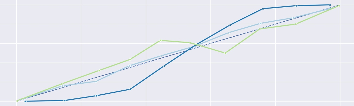
A lot is happening there.

As you can see, the logistic regression is very close to the diagonal line denoting perfect calibration. Same goes for the Keras model (called Sequential here). The curve for the random forest model has a characteristic S-shape, while the H2ODeepLearningEstimator is a slightly less smooth, reverse "S". Interestingly, the naive Bayes classifier produced a very irregular curve and the highest Brier score of all the models.

Looking at the second plot, it can be observed that the distribution of predictions has two peaks near 0 and 1 with few responses in-between. This most likely results from the relative simplicity of this particular classification task, which results in every model being pretty confident about most of the examples and returning values near the boundaries for them.

Calibrating

For the purpose of this post, we'll perform calibration ourselves, however, some frameworks and libraries support calibration out of the box. If that's the case, it's best to use these official implementations when possible as they are usually well maintained and require less effort. For the frameworks presented in this post, you should consider:

• Sklearn: CalibratedClassifierCV, which allows you to calibrate any sklearn model easily. The calibration method can be either Platt scaling or isotonic regression,
• H2O: Some models accept calibrate_model parameter, but not all of them (you can read more here).
• Keras: No official utilities, but there exist open-source projects like Calibration of Neural Networks, which you may find useful,

If you can't find the implementation that fits your needs, or simply want to experiment, consider using the approach used in this post.

We've already defined the calibrate method, so all we have to do is call it for each model, passing the calibration dataset as an argument:

for model in models:
    model.calibrate(X_calib, y_calib)

With the models calibrated, it's now possible to call predict_calibrated and calibrate_probabilities methods from our model wrappers. First, let's recheck the calibration plots and predictions distribution for "isotnic" as the calibration method.

plot_calibration_details_for_models(models, X_calib, y_calib, calibrated=True, method="isotonic")
plt.show()

We can see that the Brier scores decreased for three models and stayed similar for two of them (LogisticRegression and Sequential, which were decently calibrated from the get-go). The curves are now much closer to the diagonal line.

We'll use some extra plotting utility methods to delve deeper into calibration details for some of the models. The code below displays calibration curves for uncalibrated responses (by passing the result from predict as predicted probabilities) and then plots calibrated outcomes (with predict_calibrated) for all the models and both calibration methods. The fitted regression lines used for calibration are displayed as well, with the help of calibrate_probabilities method.

for model in models:
    plt.figure(figsize=(5, 4))
    prob_true, prob_pred = plot_calibration_curve(y_calib, model.predict(X_calib), f'{model.name} before calibration')
    plt.show()
    for method in ['sigmoid', 'isotonic']:
        plt.figure(figsize=(10, 4))
        plt.subplot(1,2,1)
        plot_fitted_calibrator(prob_true, prob_pred, model.calibrate_probabilities(prob_pred, method), f'Fitted {method} calibrator')
        plt.subplot(1,2,2)
        plot_calibration_curve(y_calib, model.predict_calibrated(X_calib, method), f'After calibration with {method}')
        plt.show()

This code produces five plots for each model, yielding 25 plots in total. To keep things shorter, we'll analyse the plots for just three models - sklearn's LogisticRegression with H2O's H2ONaiveBayesEstimator and H2ODeepLearningEstimator.

First, the logistic regression:

As can be seen, the model is almost perfectly calibrated from the beginning. In fact, calibrating it with Platt scaling (the second row) does the opposite of the desired outcome as the calibration visibly decreased. Isotonic regression (the third row) works better, but the difference is not very significant. Our results show that, for such a model, there's really no need to perform any calibration at all.

Now, let's look at the naive Bayes classifier:

The calibration curve is a bit wild for this one. It's not really an S-shaped plot, so there's no reason to expect much from Platt scaling, but we can observe that it actually improved the calibration by a fair amount (the Brier score got reduced from 0.249 to 0.215). Notice how the curve shortened a lot - this is due to the fact that the fitted sigmoid (in red colour) effectively reduced the range of possible probabilities of this classifier to something near the range of [0.45-0.6].

When it comes to the isotonic regression, we can see that the results are even better. The score got reduced even more, and, interestingly, the range of possible probabilities is broader than with the Platt scaling.

Lastly, the H2ODeepLearningEstimator - a neural network implemented in H2O library:

This one is interesting since the calibration curve is more or less a reversed "S" shape. We can reason from this, that calibrating with the sigmoid method shouldn't yield satisfactory results, and, to no surprise, it turned out to be the case. Actually, Platt scaling did the opposite of what we wanted - the model is even more miscalibrated, which is indicated by the increased value of the Brier score. Yet again, calibrating with isotonic regression proved superior, with the resulting curve pretty close to the diagonal line, and a reduced Brier score.

One last thing before we wrap up. At the beginning of the post, I mentioned that calibration can impact the accuracy of the model, although it rarely makes a significant difference. To verify this claim, let's run the following code, which calculates a set of accuracies for each model - its bare version and after calibrating with both methods discussed:

for model in models:
    accuracy = model.score(X_valid, y_valid)
    print(model.name)
    print(f'Accuracy: {round(100*accuracy, 2)}%')
    for method in ['sigmoid', 'isotonic']:
        accuracy = model.score_calibrated(X_valid, y_valid, method)
        print(f'Accuracy after {method}: {round(100*accuracy, 2)}%')
    print()

Output:

>>> LogisticRegression
>>> Accuracy: 89.77%
>>> Accuracy after sigmoid: 89.77%
>>> Accuracy after isotonic: 89.86%

>>> RandomForestClassifier
>>> Accuracy: 97.78%
>>> Accuracy after sigmoid: 97.72%
>>> Accuracy after isotonic: 97.72%

>>> H2ONaiveBayesEstimator
>>> Accuracy: 75.12%
>>> Accuracy after sigmoid: 75.2%
>>> Accuracy after isotonic: 75.12%

>>> H2ODeepLearningEstimator
>>> Accuracy: 98.65%
>>> Accuracy after sigmoid: 98.66%
>>> Accuracy after isotonic: 98.72%

>>> Sequential
>>> Accuracy: 98.34%
>>> Accuracy after sigmoid: 98.34%
>>> Accuracy after isotonic: 98.23%

As can be seen, the values fluctuate a bit, but the difference is negligible. This means that, with calibration, we achieved models outputting more meaningful responses without impacting their performance. This looks like an absolute win!

Summary

In this post, we've gone through the theoretical basis of model calibration, discussed the importance of understanding whether a classifier is calibrated or not, and implemented a simple framework for calibrating models regardless of their inner implementation. Having a good grasp of calibration is a necessity for the meaningful interpretation of numerical outputs of machine learning classifiers. With their probabilities calibrated, models gain new predictive powers - it's too enticing of a prospect to pass it over.